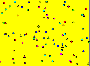
Ranked set sampling, originally developed by McIntyre (1952), combines simple random sampling with the field investigator's professional knowledge and judgment to pick places to collect samples. Alternatively, field screening measurements can replace professional judgment when appropriate. The use of ranked set sampling increases the chance that the collected samples will yield representative measurements. This results in better estimates of the mean as well as improved performance of many statistical procedures such as testing for compliance with risk-based or background-based (reference-based) standards.
Moreover, ranked set sampling can be more cost-efficient than simple random sampling because fewer samples need to be collected and measured. The use of professional judgment in the process of selecting sampling locations is a powerful incentive to use ranked set sampling. Professional judgment is typically applied by visually assessing some characteristic or feature of various potential sampling locations in the field, where the characteristic or feature is a good indicator of the relative amount of the variable or contaminant of interest that is present.
A simple ecological example will illustrate the ranked set sampling method. Suppose the average age of trees on a property needs to be estimated. An appropriate judgment-based measurement (the visual size of a tree - trees generally increase in size as they age) exists. Begin by randomly selecting three trees and judge by eye which tree is the smallest. Mark the smallest tree to be measured and ignore the other two. Next, randomly select another set of three trees to rank. Mark the medium sized tree and ignore the other two. Next, randomly select another three trees. Mark the largest tree and ignore the other two. Repeat this procedure 10 times (10 cycles) for a total of 90 trees. 30 of the trees will have been marked and 60 ignored. Of the 30 marked trees, 10 are from a stratum of generally smaller trees, 10 are from a stratum of generally middle-sized trees and 10 are from a stratum of generally larger trees. Determine the age of each of the 30 marked trees by coring or some other appropriate measurement technique and use that measurement to estimate the average age of the trees on the lot.
In this illustration there were 10 cycles and 3 samples chosen per cycle. In practice, the number of sample locations chosen per cycle (the "set size") and the number of cycles is determined using a systematic planning process. Visual Sample Plan implements the systematic process needed to determine the number of cycles, and hence, the number of locations to be ranked and the number of locations to be measured. VSP can also place ranking and sampling locations on the map of the study site.
Ranking Cost per Location: 25.00
Lab Data Distribution: Symmetric
Ranking Method: Professional Judgment
Set Size: 3
Choose: Two-sided Confidence Interval About the Mean
Confidence Level: 95%
Maximum acceptable half-width of confidence interval: 5.5
Estimated Standard Deviation: 20
Chosen set size (m): 3
Number of cycles (r): 10
Required number of samples (m x r): 30
Number of field locations to rank (m x m x r): 90

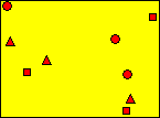
The squares represent the first set of field locations. The three trees closest to these locations on the map would be judged and the smallest tree would be chosen for sampling (coring or some other method). The triangles represent the second set of field locations. The three trees closest to these locations on the map would be judged and the medium-sized tree would be chosen for sampling. Finally, the circles represent the third set of field locations in the first cycle. The three trees nearest these locations on the map would be judged and the largest tree would be sampled.
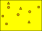
The same process would be repeated for all 10 cycles. At the end of the 10 cycles, you will have collected 30 samples, 3 from each cycle. The mean age given by these samples will have a 95% probability of being within 5.5 years of the actual mean age of the trees on this property (if your assumptions are reasonable: 20 year standard deviation, etc.)
Suppose that it has been noted that more of the trees are older than younger, making the population skewed toward higher ages. This would indicate the need for an unbalanced ranked set sampling design. In an unbalanced design, the top rank may be sampled more than once in order to better determine the mean when more values in the population are near the top of the distribution.
Ranking Cost per Location: 25.00
Lab Data Distribution: Asymmetric (Skewed toward High)
Ranking Method: Professional Judgment
Set Size: 3
Confidence Level: 95%
Maximum acceptable % difference between estimated mean and true mean: 15
Geometric Standard Deviation: 1.5
Chosen set size [m]: 3
Number of cycles [r]: 6
Number of sets for top rank [t]: 2
Number of sets per cycle [m+t-1]: 4
Required number of samples [(m+t-1) x r]: 24
Number of field locations to rank [(m+t-1) x m x r]: 72
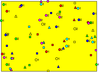

The squares represent the first set of field locations. The three trees closest to these locations on the map would be judged and the smallest tree would be chosen for sampling (coring or some other method). The triangles represent the second set of field locations. The three trees closest to these locations on the map would be judged and the medium-sized tree would be chosen for sampling. The circles represent the top rank. Notice that there are two sets of circles: one set accompanied by the numeral 1 and the other set accompanied by the numeral 2. This is because the top rank has to be sampled twice for this unbalanced design (t = 2). The circle-1s represent the third set of field locations in the first cycle. The three trees nearest these locations on the map would be judged and the largest tree would be sampled. Finally, the circle-2s represent the fourth set of field locations in the first cycle. The three trees nearest these locations on the map would be judged and, again, the largest tree would be sampled.
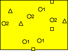
The same process would be repeated for all 6 cycles. At the end of the 6 cycles, you will have collected 24 samples, 4 from each cycle. The mean age given by these samples will have a 95% probability of being within 15% of the actual mean age of the trees on this property (if your assumptions are reasonable: 1.5 geometric standard deviation, etc.)
There are 2 major design types for RSS: balanced and unbalanced designs. Balanced designs assume that the analytical measurements of interest are symmetrically distributed about the mean. Unbalanced designs assume that the distribution of measurements is skewed to higher values. Unbalanced designs select more samples from the top rank to better estimate the mean given the skewness of the data.
Determining the number of cycles, and hence, the number of locations to be ranked and the number of locations to be measured, is a 5 step process:
For balanced designs, the number of samples needed for simple random sampling (\(n_0\)) is calculated by VSP using either a one-sided or a two-sided confidence interval equation, as selected by the VSP user.
For a two-sided confidence interval, the equation used to calculate the number of samples under simple random sampling, \(n_0\), when the expected distribution is symmetric and a balanced ranked set sampling design is used is: $$n_0 = s^2\Bigg(\frac{t_{1-\alpha/2, df}}{d}\Bigg)^2$$
For a one-sided confidence interval, the equation used is: $$n_0 = s^2\Bigg(\frac{t_{1-\alpha, df}}{d}\Bigg)^2$$
where
\(n_0\) |
is the recommended minimum number of samples for the study area if simple random sampling were used, |
\(s\) |
is the estimated standard deviation of measurements of collected samples, |
\(d\) |
is the maximum desired width (or half-width) of the confidence interval, |
\(t_{1-\alpha,df}\) |
is the value of the Student's t-distribution with \(n\)-1 degrees of freedom (df) such that the proportion of that distribution less than \(t_{1-\alpha,df}\) is \(1-\alpha\), and |
\(t_{1-\alpha/2,df}\) |
is the value of the Student's t-distribution with \(n\)-1 degrees of freedom (df) such that the proportion of that distribution less than \(t_{1-\alpha/2,df}\) is \(1-\alpha/2\). |
Because \(n\) appears on both sides of the above equations (on the right side it appears in the degrees of freedom of the t-distribution), the equation must be solved iteratively. VSP does this automatically using the iteration scheme in (Gilbert 1987, pg. 32).
For unbalanced designs, the number of samples is computed using the Adjusted Classical Formula method outlined by (Perez and Lefante 1997).
Using this method, the first step is to compute an approximate sample size using the following formula: $$n_{\text{classic}} = \Bigg(\frac{Z_{1-\alpha/2}}{\pi}\Bigg)^2(GSD^{ln(GSD)}-1)$$
where
\(n_{\text{classic}}\) |
is the approximate recommended minimum number of samples, |
\(Z_{1-\alpha/2}\) |
is the value of the standard normal distribution such that the proportion of the distribution less than \(Z_{1-\alpha/2}\) is \(1-\alpha/2\), |
\(GSD\) |
is the geometric standard deviation, |
\(ln\) |
is the natural logarithm, and |
\(\pi\) |
is the maximum proportion difference between the estimated mean and the true mean. |
Next, linear regression is used to calculate the recommended minimum number of samples using the following formula: $$n_0 = \beta_0 + \beta_1(n_{\text{classic}})$$
where
\(n_0\) |
is the number of samples required under simple random sampling, |
\(\beta_0\) |
is the Y-intercept of the regression formula, |
\(\beta_1\) |
is the slope of the regression formula. |
\(\beta_0\) is obtained from the following table [from Table III in (Perez and Lefante 1997, pg.2791)]:
Confidence Level |
GSD = 1.1 |
GSD = 1.5 |
GSD = 2.0 |
GSD = 2.5 |
GSD = 3.0 |
GSD = 3.5 |
GSD = 4.0 |
90% |
2.9532 |
7.5249 |
11.3183 |
15.5638 |
20.1322 |
25.9327 |
30.3223 |
95% |
3.3331 |
7.9237 |
14.0744 |
20.5406 |
27.1563 |
33.6865 |
40.1084 |
99% |
4.9265 |
11.2470 |
20.5069 |
30.2478 |
40.1743 |
51.1945 |
60.6576 |
\(\beta_1\) is obtained from the following table [from Table III in (Perez and Lefante 1997, pg.2791)]:
Confidence Level |
GSD = 1.1 |
GSD = 1.5 |
GSD = 2.0 |
GSD = 2.5 |
GSD = 3.0 |
GSD = 3.5 |
GSD = 4.0 |
90% |
0.4714 |
0.6926 |
0.8509 |
0.8794 |
0.8499 |
0.7731 |
0.7033 |
95% |
0.4726 |
0.8094 |
0.9046 |
0.9129 |
0.8731 |
0.8072 |
0.7288 |
99% |
0.4740 |
0.8865 |
0.9808 |
0.9877 |
0.9444 |
0.8612 |
0.7796 |
This value is usually based on practical constraints in ranking locations in the field using professional judgment or field screening measurements. It may be difficult to use professional judgment to accurately rank by eye more than 4 or 5 locations. Other constraints that may affect the size of m are time, staff, and cost considerations. VSP limits m to 5 for judgment sampling and 8 for field screening measurements.
Relative precision is needed to calculate the number of cycles. For balanced designs, relative precision RP is found from the following table assuming the data are normally distributed [from Table 1 of (Patil et. al. 1994, pg.176)]:
Set Size = 2 |
Set Size = 3 |
Set Size = 4 |
Set Size = 5 |
1.467 |
1.914 |
2.347 |
2.770 |
If the set size, m, is greater than 5, RP is found using the following linear formula:
\(RP = 0.4342m + 0.6048\)
For unbalanced designs, RP is found from the following table , assuming the data are lognormally distributed [from Table 1 of (Patil et. al. 1994, pg.177)]:
Set Size |
CV = 0.1 |
CV = 0.202 |
CV = 0.307 |
CV = 0.416 |
CV = 0.533 |
CV = 0.658 |
CV = 0.795 |
CV = 0.947 |
CV = 1.117 |
CV = 1.311 |
2 |
1.46 |
1.45 |
1.42 |
1.40 |
1.37 |
1.33 |
1.29 |
1.26 |
1.22 |
1.19 |
3 |
1.90 |
1.87 |
1.83 |
1.77 |
1.70 |
1.62 |
1.55 |
1.47 |
1.40 |
1.34 |
4 |
2.33 |
2.28 |
2.21 |
2.11 |
2.00 |
1.89 |
1.78 |
1.67 |
1.56 |
1.47 |
5 |
2.75 |
2.68 |
2.57 |
2.44 |
2.29 |
2.14 |
1.99 |
1.84 |
1.71 |
1.59 |
6 |
3.15 |
3.07 |
2.93 |
2.76 |
2.57 |
2.37 |
2.18 |
2.00 |
1.84 |
1.70 |
7 |
3.56 |
3.45 |
3.28 |
3.07 |
2.83 |
2.60 |
2.40 |
2.16 |
1.96 |
1.80 |
8 |
3.95 |
3.86 |
3.61 |
3.36 |
3.09 |
2.81 |
2.55 |
2.30 |
2.08 |
1.89 |
CV is the coefficient of variation found by computing:
\(CV = \sqrt{e^{ln(GSD)^2}-1}\),
which assumes the data are lognormally distributed.
Number of cycles, \(r\), is found with the following formula:
\(r=\frac{n_0/m}{RP}\)
For balanced designs, the total number of samples, \(n\), is found simply by the following formula:
\(n = r*m\)
The number of field locations that need to be ranked to get the \(n\) samples is:
\(r*m*m\)
For unbalanced designs, the number of times, \(t\), the top rank needs to be sampled is found from the following table (from Table 8-5 in QA/G-5S):
CV |
0.25 |
0.5 |
1.0 |
1.25 |
1.5 |
2.0 |
2.5 |
3.0 |
3.5 |
4.0 |
\(t\) |
1 |
2 |
3 |
4 |
5 |
6 |
7 |
8 |
9 |
10 |
The total number of samples, \(n\), is found by the following formula:
\(n = rx(m+t-1)\)
The number of field locations that need to be ranked to get the n samples is:
\(r*m*(m+t-1)\)
For ranked set sampling, VSP produces field sample markers on the map that have different shapes and colors.
The color of the marker indicates its cycle. The cycle colors start at red and go through the spectrum to violet. Use the Cycle drop list on the Ranked Set Sampling Toolbar to show only the field locations for a particular cycle.
The shape of the marker indicates its set. Field sample locations for the first set are marked with squares, locations for the second set are marked with triangles, etc. For unbalanced designs, the top set is sampled several times, so a number accompanies those markers. Use the Set drop list on the Ranked Set Sampling Toolbar to show only the field locations for a particular set.
Ranked set field sampling locations are generated with a label having the following format:
\(RSS- c-s-i\)
where
\(c\) indicates the cycle number
\(s\) indicates the set number (for unbalanced designs this number is also incremented for each iteration of the top set)
\(i\) is a unique identifier within the set
Use the View Labels command on the menu or the Toolbar to show or hide the labels for the field sampling locations.
The assumptions used to determine the number of balanced ranked set samples are:
1. The sample mean is normally distributed (used to compute \(n_0\)).
2. The variance estimate, \(s^2\), is reasonable and representative of the population being sampled (used to compute \(n_0\)).
3. The data distribution is symmetric and approximately normally distributed (used to determine RP).
4. The estimate of the sample mean is reasonable and representative of the population being sampled.
5. The field locations that will be ranked are selected using simple random sampling.
The first three assumptions will be assessed in a post data collection analysis. The fourth assumption is valid because the sample mean will be an unbiased estimate of the population mean. It is the responsibility of the investigators to ensure that the fifth assumption is met.
For an illustration on ranked set sampling, please refer to Ranked Set Sampling in chapter 3 of the VSP User’s Guide.
EPA, November 2001. Guidance for Choosing a Sampling Design for Environmental Data Collection, EPA QA/G-5S, Peer Review Draft, Washington, D.C.
Gilbert, R.O. 1987. Statistical Methods for Environmental Pollution Monitoring. John Wiley & Sons, NY.
McIntyre, G.A. 1952. A method for unbiased selective sampling using ranked sets, Australian Journal of Agricultural Research 3:385-390.
Patil, G.P., A.K. Sinha and C. Taillie. 1994. Ranked set sampling, Handbook of Statistics 12, Environmental Statistics, pp. 167-200, (G.P. Patil and C.R. Rao, editors), North-Holland, New York, NY.
Perez, A., and J.J. Lefante. 1997. Sample size determination and the effect of censoring when estimating the arithmetic mean of a lognormal distribution. Communications in Statistics, Theory and Methods 26 (11):2779-2801.
Analysis / Screening Correlation
For One-Sided Confidence Interval :
Maximum Acceptable Width of Confidence Interval
For Two-Sided Confidence Interval :
Maximum Acceptable Half-Width of Confidence Interval
Maximum acceptable % difference between estimated mean and true mean
See also: Ranked Set Sampling Toolbar