Geophysical surveys are conducted at DoD sites and facilities to search for Target Areas at which munitions were fired or dropped. Surface areas passed over by geophysical detectors, referred to as transects, are usually up to several meters wide, and run in a relatively straight line (as much as terrain permits) from one point of a site to another. When a geophysical sensor system is deployed continuously along transects, anomalous readings may be recorded. A goal of these surveys is to identify areas of high anomaly density consistent with that of a target area. The methods in VSP are statistical approaches for determining the level of confidence that a transect sampling design will traverse and/or detect a target area of a specific shape, size, and anomaly density.
This module in VSP allows either the distance between transects or the target area's anomaly density to be fixed while the other is analyzed over a range of possible values. Analyzing a range of distances between transects allows for a statistically defensible choice of transect spacing based on the probability of detecting and/or traversing the target area. Analyzing a range of target area anomaly densities provides confidence estimates of how well a given sampling design will work for target areas of different densities.
Transects patterns available are parallel, square, and rectangular. In parallel patterns, transects run parallel across the site and are spaced equally apart. In square patterns and rectangular patterns, two parallel patterns are used with their respective transects running perpendicular to transects in the other pattern. In rectangular patterns, the spacing of transects is different between the two patterns.
Transect patterns: Parallel (left), Square (middle), and Rectangular (right)
The transect width, which is dependent on the sensor footprint, is the width of the area on the ground surface for which the geophysical detector passes over and collects data. Units can be entered in feet, meters, or inches. The transect width along with the transect's length determine the amount of surface area a transect covers.
There are two major ways to define the target size and shape: manually enter the size and shape parameters or have VSP calculate the size and shape from built in model tables.
Choose this option to allow VSP to set the size and shape based on some munitions modeling. After choosing this option, there are several choices including Surface launched / Air launched, High Explosive / Chemical, etc. See Simplified Target Sizing Model for Visual Sample Plan (Hathaway 2013) for more details.
Different options are available for entering the size and shape of the target area. Options include entering the major axis and minor axis, entering the major axis and shape, or entering the area of the target and shape. There is also an option for fixing the angle of the target in relation to transects, or allowing this to be random (the default). These parameters are further explained below.
The area of the target is the total surface area over which the target area lies. Units can be entered in square feet, square meters, square inches, or acres.
The target area is assumed to be circular or elliptical. The semi-major axis, \(r_x\), is the distance from the target area's center to its perimeter at its widest point, or one-half the major axis, as shown in the illustration below. For a circle, this is simply the circle's radius.
The semi-minor axis, \(r_y\), is the distance from the target area's center to its perimeter at its narrowest point, or one-half the minor axis, as shown in the illustration above. For a circle, the semi-major axis is equal to the semi-major axis. The semi-minor axis is never greater than the semi-major axis.
The shape of the target is the ratio of the semi-minor axis to the semi-major axis. The shape will never be greater than 1, and has a lower-limit of 0.2 since target areas do not tend to be any narrower than this. When the shape is changed, the semi-minor axis is adjusted so that it has the correct ratio with the semi-major axis. The area of the target area is also adjusted.
When the target area is elliptical, an option is available to fix the angle of the target area's major axis in relation to the transects by clicking on Degrees and entering the angle in degrees. This may be used when information is available about the angle of the target area's semi-major axis at the site, such as knowing the specific direction in which ordnance was being fired. It is recommended that the Random option be used unless very reliable information is known about this angle. If the angle is known with near certainty, then entering the angle will result in a transect design with a reduction in the number of transects needed to traverse the target area or reduce some of the uncertainty in the estimate of the probability of detection.
Three different design objectives are available and are explained below. Parameters shown directly below the Design Objective dropdown are explained within the details of each design objective below. Other parameters that apply to the design objectives are explained later in the Target Detection Performance section.
This design objective focuses on developing a sampling design for which VSP's target detection methods will have a high probability of detecting potential target areas. In the Target Detection Performance section of the Transect Spacing tab, there is a drop-list with an option to choose between TA density (above background) range or Transect spacing evaluation range. Choosing the TA density option allows for VSP to conduct a sensitivity analysis for the ability of a fixed sampling design to detect the target area for a range of target area densities. Choosing the Transect spacing option allows for VSP to conduct a sensitivity analysis for the ability of a range of transect spacings to detect a target area with specified density. This design objective uses parameters from the Survey & Target Area Pattern tab as well parameters on the Transect Spacing tab.
This design objective focuses only on the probability that at least one transect will traverse the target area. When selected, the next parameter on the screen is Required Probability of Traversing Target, for which the required probability of having one or more transects traverse the target is entered. The required space between transects is returned (printed in red text in the dialogue) based on this input and the defined transect width and target area in the Survey & Target Area Pattern tab.
Required Probability of Traversing Target
This parameter is only available when the Design Objective is set to Ensure high probability of traversal only (see the explanation of this Design Objective above). A percentage is entered and the required space between transects is printed below in red text.
The purpose of this option is to make available some of VSP's useful features, such as overlaying transect locations on a site map and exporting transect coordinates to a text or .SHP file. Before deciding to develop a sampling plan based on a user-supplied transect spacing and starting location, consider the assumptions and limitations involved, as detailed in this help file.
Transect Spacing
The user enters the spacing between transects for the transect design.
Starting Location
Two options are available for starting location, entering X-Y coordinates or using a random start. When X-Y coordinates are selected and entered, it is assumed a transect will pass through those points. Otherwise, random start will assume the transect locations or starting point is random.
The background density, \(D_b\), of a site is the expected density in an area where anomalies occur solely from geologic material or anthropogenic clutter not related to DoD range activities. These background anomalies are treated as though they are uniformly distributed throughout the site. Areas containing UXO and other munitions-related anomalies are expected to have density greater than background. Background density is a critical parameter since ultimately we are trying to detect these areas of elevated density. Background density can be entered as the number of anomalies for square feet, square meters, square inches, or acres.
The Decision Rule is the required percent confidence that an area has density greater than background density needed to conclude it is an area of interest. VSP evaluates a number of windows, which are circular areas centered along transects. The Decision Rule refers to the percent confidence for an individual window. VSP will flag an area that appears to have density higher than background density according to the decision rule. An area is flagged if the actual density is significantly higher than the expected background density. In statistical terms, the decision rule is \(1 - \alpha\) expressed as a percentage, where \(\alpha\) is the probability of a type I error, or the probability of concluding an area has density greater than background when it is truly a background area.
The false negative detection error rate, \(P_{fn}\) , accounts for the fact that collected data may not be representative of the actual density because the geophysical detector may not always detect an individual detectable anomaly. For example, a false negative rate of 5% would indicate the detector, on average, would fail to detect 5% of the total anomalies traversed. If it were assumed that the detector always detects individual anomalies, then a false negative rate of 0% would be used.
When this option is selected, the user enters a range of possible target area densities in the min and max fields for use in the sensitivity analysis where the probability of detecting the target area is estimated for the range of target area densities.
When TA density (above background) range is selected, this field appears. The user must enter the transect spacing they would like to evaluate.
This option is available when the design objective is set to Ensure high probability of traversal and detection. When this option is selected, the user enters a range of possible transect spacings in the min and max fields. VSP estimates the probability of detecting the target for this range of transect spacings to help choose an appropriate transect spacing.
When Transect spacing evaluation range is selected, this field appears. The user must enter the difference (greater than 0) between the average expected density of the target area and the background density. This is the expected target area density above the background density.
There are two options for specifying the distribution of the density above background in the target area, uniform density and bivariate normal density. The minimum precision, maximum error, and Search Window Diameter affect the length of the Monte Carlo simulations which estimate the probability of detecting the target area. These distributions and parameters are explained below.
When Uniform Density is selected, the additional ordnance-related anomalies in the target area are assumed to have a uniform distribution, meaning they are spread equally through the target area.
When Bivariate Normal Density is selected, the additional ordnance-related anomalies in the target area are assumed to have a bivariate normal distribution, meaning they are more concentrated towards the center of the target area and are sparse near the target area's perimeter. An example of a bivariate normal distribution is shown in the illustration below.
By default, the average density above background density for the target area is entered, DTA. When Bivariate Normal Density is selected, there are two other options other than entering the average density which are explained below. These are the density at the outer edge of the target or at the target's center.
When this option is selected, the density above background density for the target is assumed to be the density at the target edges (see illustration above) rather than the target area's average.
When this option is selected, the density above background density for the target is assumed to be the density at the target center (see illustration above) rather than the target area's average.
Minimum Precision is used to determine the number of different TA densities or transect spacings to simulate. Initially the highest and lowest values of the user specified range are simulated. For example, if transect spacings are being simulated between 100m and 200m, then simulations are initially done using transect spacings of 100m and 200m. The difference of the probabilities is calculated, and if it is greater than the minimum precision, another iteration is run using the average of the highest and lowest values in the user specified range of densities or transect spacings. This process is repeated for all pairs of adjacent transect spacings or densities simulated until no pair has a difference in probability of detection greater than the minimum precision. Decreasing the minimum precision typically increases the length of the simulation, and increasing the minimum precision typically decreases the length of the simulation.
Maximum Error determines the number of iterations for each transect spacing or density simulated. A minimum number of iterations is run to begin the simulation and then additional iterations are run until the Maximum Error is satisfied. If the total number of iterations after an iteration is \(n\) and the proportion of TAs detected is \(p\), then another iteration is run if
$$ Maximum Error < 1.96 \times \sqrt{\frac{p(1-p)}{n}} $$
The quantity \(1.96 \times \sqrt{\frac{p(1-p)}{n}}\) is the 95th percentile of the standard error of the mean for a binomial distribution. We are 95% certain that the estimated probability is close to the true probability (within the maximum error). Decreasing the maximum error typically increases the length of the simulation. Increasing the maximum error typically decreases the length of the simulation.
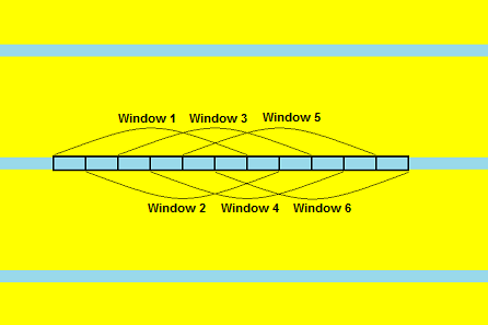
A rectangular search window is used to identify areas where anomaly density is greater than background density, and the length of this search window can be specified. The window is actually a moving window that moves in increments of 1/6 the window length along each transect. An example of six successive search windows along a transect is shown in the illustration below. Each search window will be evaluated to determine if the density is significantly greater than background density.
Below the search window entry box, the critical number of anomalies is displayed. This is the number of anomalies in a search window that indicates the density is significantly greater than background density. VSP will default to a search window length of 90% of the target diameter (for circular target areas), or 90% of the target minor axis (for elliptical target areas). The user can specify the search window length by checking the Over-ride box and manually entering the desired length.
Checking this option will display additional power curves on the plot to examine both sensitivity to target area density and transect spacing at the same time. This will increase the simulation run time since it requires additional simulations.
To generate an estimated probability on a graph, VSP runs a Monte Carlo simulation based on the entered parameters. For each iteration, VSP creates a square site with center at the origin (0,0), and sides of approximate length \(2r_x + 2r_w\). A parallel transect pattern is placed randomly so that transects are parallel to the x-axis. In a square or rectangular pattern, the additional transects will be randomly placed so they are parallel to the y-axis. The TA is centered at the origin (0,0) and rotated at a random angle \(\theta\) where \( 0 \leq \theta \leq \pi\) radians.
VSP calculates the total area of the site traversed by transects,\(A_b\). The expected number of detected background anomalies,\(\lambda_b\), is calculated as \(\lambda_b = D_b A_b (1 - P_{fn})\). A random number of detected background anomalies is generated using a Poisson distribution with parameter \(\lambda_b\). VSP randomly places these anomalies within the traversed areas of the site.
For a target area of surface area \(A_t\) with a uniform density above background, the number of non-background anomalies within the target area needed to achieve the user specified density is calculated as \(n_d = A_tD_{TA} \), with VSP rounding \(n_d\) up to the nearest integer. VSP then randomly selects the number of non-background anomalies that would be detected with a single pass of the geophysical sensor by generating a random Binomial variable,\(n_e\), with parameters \(n_d\) and \( 1 - P_{fh}\), and randomly places \(n_e\) anomalies within the target area. Anomalies not traversed by a transect are deleted. This simulates the number of objects detected within the target area.
For a target area with a bivariate normal density above background, VSP places a string of points spaced apart by the transect width along the portion of each transect that traverses the TA. These center points are centered on each transect's center line. For each center point, VSP calculates the distance from the TA center, \(d_f\), the distance from the TA center to the TA perimeter through this center point, \(d_p\), and the fraction of the TA's area inside the quantile on which the center point lies, \(d_{ratio} = \left( \frac{d_f}{d_p} \right)^2 \). We assume that the spatial coordinates (locations) of detectable items in the elliptical TA have a bivariate normal distribution. Then, \(l = \dbinom{x}{y}\) and \(l \sim N(\mu , \Sigma )\), where \( \mu = \dbinom{\mu_x}{\mu_y}\) and \(\Sigma = \dbinom{\sigma_x^2 \quad \rho \sigma_x \sigma_y}{\rho \sigma_x \sigma_y \quad \sigma_y^2}\). The quadratic form \(l'\Sigma^{-1} l\) is known to have a Chi-Square \(\chi^2\)) distribution with 2 degrees of freedom; i.e., \(l'\Sigma^{-1} l \sim \chi_2^2 \). In VSP, the boundary of the TA is defined to be 99th quantile of the bivariate normal distribution. VSP divides the TA up into 99 quantiles which all have an equal number of expected detectable anomalies, but the area in these quantiles increases according to a \(\chi_2^2\) distribution. This robustly approximates the \(\chi^2\) distribution. Therefore, the \(i^{th}\) quantile has average density \( \large \frac{D_{TA} A_t}{99} \times \frac{\chi_{0.99,2}^2}{A_t (\chi_{i / 100,2}^2 - \chi_{(i-1)/100,2}^2)} = \frac{D_{TA} \chi_{0.99, 2}^2}{99( \chi_{i/100,2}^2 - \chi_{(i-10)/100,2}^2)} \). VSP determines the quantile in which each center points lies and assigns the corresponding non-background density to the square-shaped area. The expected number of anomalies within this area is computed and multiplied by (\(1 - P_{fn}\)) to determine the expected number of detected anomalies. A random number of detected anomalies is generated according to a Poisson distribution, and the anomalies are randomly placed within the square-shaped area. For square and rectangular patterns, non-background anomalies in areas where transects overlap are deleted if they originated from a center point on a transect parallel to the y-axis.
VSP places a string of points on each transect spaced \(\frac{r_w}{3}\) apart. These points are the centers of all rectangular search windows available for analysis. The traversed area, \(a_w\), is calculated and used as the traversed area for all windows. The number of detected anomalies, \(n_a\), is calculated within a window. Using \(a_w\) and \(n_a\) the density of the window, \(D_a\), is calculated. For each window, the null and alternative hypotheses for determining if the area inside the window has density significantly greater than background density, \(D_b\), are as follows:
Null Hypothesis: \(H_0 : D_a \leq D_b\)
Alternative Hypothesis: \(H_0 : D_a > D_b\)
Initially we assume that each window does not intersect the target area. Given this assumption, the distribution of \(n_a\) is Poisson with parameter \(\lambda = D_b A_w (1 - P_{fn})\). For \(n_a = 0\), VSP determines the density at the coordinates is not significantly greater than \(D_b\) since no anomalies were detected. For \(n_a \geq 1\), VSP determines the density at the coordinates is significantly greater than \(D_b\) if \( \left( 1 - \displaystyle\sum_{i=0}^{n_a - 1} \frac{e^{- \lambda} \lambda^i}{i!} \right) < \alpha \) where \( \left(1 - \displaystyle\sum_{i=0}^{n_a - 1} \frac{e^{- \lambda} \lambda^i}{i!} \right) < \alpha \) is the probability of detecting \(n_a\) or more anomalies within an area of size \(a_w\) and with density \(D_b\). If the density of a window is significantly greater than the background density, it is assumed that the TA has been detected, and the remaining windows are not checked. The iteration stops either when a window intersecting the target area is flagged as significant, or when every window has been checked.
This process is repeated until the desired maximum error is achieved. When all iterations are completed, VSP tabulates the estimated probability the TA has been detected, \( \bar P_{TD} = \frac{number \, of \, TA's \, detected}{number \, of \, simulations}\).
Shows statistics about site coverage and surveying costs.
1. The target area (its projection onto the coordinate plane) is circular or elliptical.
2. Transects are laid out in parallel, square, or rectangular patterns.
3. The transect width corresponds to the effective width of view of the sensor as it traverses the ground.
4. The density of the anomalies in the target area follows a uniform or bivariate normal distribution.
5. Transects are perfectly straight lines and spaced as computed by VSP.
Hathaway JE, BA Pulsipher, JE Wilson, and LLN Newburn. 2013. Simplified Target Sizing Model for Visual Sample Plan (VSP) - Redacted Version: Methodology for Munition Specific Fragmentation Distances for use in VSP based on TP-16 Methodology. PNNL-22394, Pacific Northwest National Laboratory, Richland, WA.
Hathaway, J, B. A. Pulsipher, J. E. Wilson, C. A. McKinstry. 2006. Final Report for Statistical Methods and Tools for UXO Site Characterization on Final Simulated Site. PNNL- 15651, Pacific Northwest National Laboratory, Richland, Washington.
Gilbert, R. O, J. E. Wilson, R. F. OBrien, D. K. Carlson, B. A. Pulsipher, and D. J. Bates. 2003. Version 2.0 Visual Sample Plan (VSP): UXO Module Code Description and Verification. PNNL-14267, Pacific Northwest National Laboratory, Richland, Washington.
Matzke BD, JE Wilson, and BA Pulsipher. 2006. Version 4.4 Visual Sample Plan (VSP): New UXO Module Target Detection Methods. PNNL-15843, Pacific Northwest National Laboratory, Richland, WA.