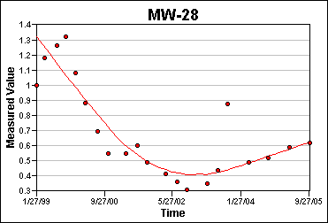

For the LOWESS (Locally Weighted Smoothing Scatterplot), VSP uses the method developed by William S. Cleveland (1979). The method, as implemented by VSP, proceeds as follows:
1. The neighborhood size, \(r\) , is computed as \(f \times N\), where \(N\) is the number of data points and \(f\) is the neighborhood scaling factor \(0 < f \leq 1\). (Note: VSP uses a default value of \(f\) = 0.5)
2. A fitted value, \( \hat y_i\), is obtained for each data point (\(x_i,y_i\)), \(i = 1..N\) using locally weighted regression:
A weight, \(W_j\), \(j = 1..N\), is calculated for each data point using the formula:
$$ W_j = Tri \left( \frac{x_j - x_i}{h} \right) $$
Where:
\(h\) is the \(r^{th}\) smallest distance \(|x_j - x_i|\), \(j = 1..N\) ,
and \(Tri(x)\) is the TriCube function:
$$ Tri = ( 1 - |x|^3)^3 , \quad \text{for} |x| < 1 $$
$$ Tri = 0 , \quad \text{for} |x| \geq 1 $$
The fitted value is computed as:
$$ \hat y_i = x_i \times slope + intercept \text{,} $$
Where \(slope\) and \(intercept\) are the results of weighted linear regression using the weights \(W_1..W_N\).
3. A robustness weight, \(\delta_i \text{,} i = 1.. N \) , is computed for each data point using the formula:
$$ \delta_i = Bi \left( \frac{|y_i - \hat y_i|}{6s} \right) $$
Where:
\(s\) is the median of the residual values \(| y_i - \hat y_i | \text{,} \quad i = 1.. N\),
and \(Bi(x)\) is the BiSquare function:
\( Bi = (1 - x^2)^2 , \quad \text{for} |x| < 1 \)
\(Bi ,\, \text{for} |x| \geq 1 \)
4. A new fitted value, \( \hat y_i \text{,} \quad i = 1.. N\), is obtained for each data point using weighted regression based on the robustness weights:
A weight, \(W_j \text{,} \, j = 1.. N\), is calculated for each data point using the formula:
$$ W_j = Tri \left( \frac{x_j - x_i}{h} \right) \delta_j $$
Where:
\(h\) is the \(r^{th}\) smallest distance \(|x_j - x_i| \text{,} \quad j = 1.. N\),
\(\delta_j\) is the robustness weight defined above,
and \(Tri(x)\) is the TriCube function defined above.
The fitted value is computed as:
$$ \hat y_i = x_i \times slope + intercept \text{,} $$
Where slope and intercept are the results of weighted linear regression using the weights \(W_1..W_N\).
5. Step 3 and 4 are performed a total of \(t\) times. (Note: VSP uses a default value of \(t\) = 2)
6. The output points \(( x_i' , y_i') \text{,} \quad i = 1.. n\), are computed as follows:
$$ x_i' = x_{min} + (i-1) \left(\frac{x_{max} - x_{min}}{n - 1} \right) $$
Where:
\(n\) is the number of output points,
\(x_{min}\) is the minimum date in the data set,
and \(x_{max}\) is the maximum date in the data set.
A weight, \(W_j \text{,} \, j = 1.. N\), is calculated for each data point using the formula:
$$ W_j = Tri \left( \frac{x_j - x_i'}{h} \right) \delta_j $$
Where:
\(h\) is the \(r^{th}\) smallest distance \(|x_j - x_i| \text{,} \quad j = 1.. N\),
\( \delta_j\) is the robustness weight defined above,
and \(Tri(x)\) is the TriCube function defined above.
The fitted value is computed as:
\( y_i' = x_i' \times slope + intercept\),
Where \(slope\) and \(intercept\) are the results of weighted linear regression using the weights \(W_1..W_N\).
The output points (\(x_i',y_i'\)) are plotted as the line for the visual display.
William S. Cleveland. Robust Locally Weighted Regression and Smoothing Scatterplots, 1979, Journal of the American Statistical Association, Vol. 74, No. 368. p. 829-836.