3.0 Sampling Plan Development Within VSP

3.1 Sampling Plan Type Selection

Sampling plan components consist of where to take samples, how many samples to take, what kind of samples (e.g., surface soil, air), and how to take samples and analyze them. We identified the general areas of where to take samples in Section 2.3, Sample Areas in VSP.  In this section, we discuss where within the Sampling Area to locate the samples. We also discuss how many samples to take. The kind of samples to take-i.e., soil vs. groundwater, wet vs. dry, surface vs. core,-is determined during Step 3 of the DQO process (Define Inputs) and is not addressed directly in VSP. The Measurement Quality Objectives module in VSP (Section 5.4) deals with how the method selected for analytically measuring the sample relates to other components of the sampling plan.

3.1.1 Defining the Purpose/Goal of Sampling

VSP follows the DQO planning process in directing users in the selection of the components of the sampling plan. The first thing you must do is to select the type of problem for which the current data collection effort will be used to resolve. In VSP, we call this the Sampling Goal. The following types of problems are addressed currently in VSP. Future versions will expand on this list:

This list of sampling goals available in VSP reflects the targeted interests and specific problems of our current VSP sponsors. Therefore, the available sampling designs within VSP are not an exhaustive list of designs you might find in a commercial statistical sampling package. Future versions will work toward a complete set of sampling design offerings.

VSP lists "Non-statistical sampling approach" under Sampling Goals, but this is not really a goal. Under this category, VSP allows the user to specify a predetermined sample size and locate the samples judgmentally. Because VSP has no way of knowing how the sample size and sample locations were chosen, the sampling approach is considered to be "non-statistical" (i.e., no confidence can be assigned to the conclusions drawn from judgment samples).

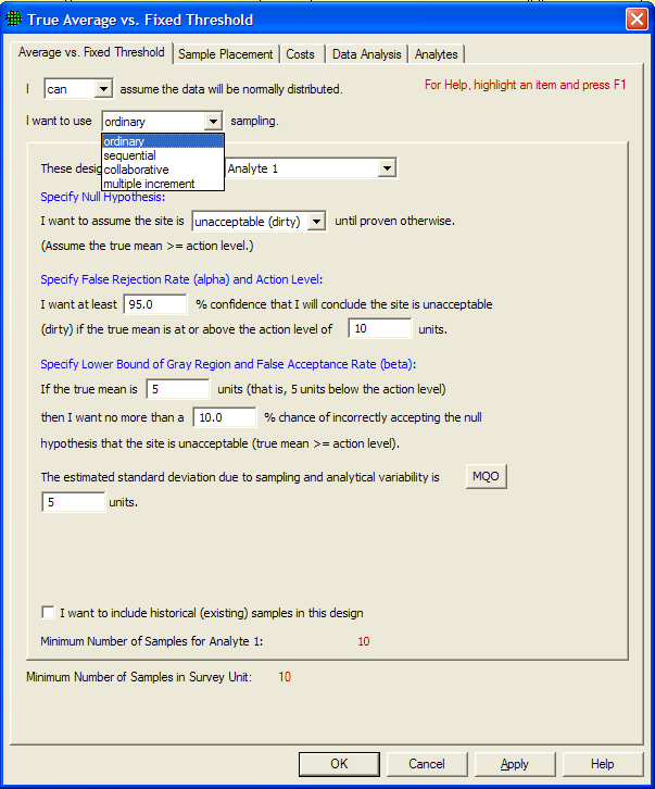
To give you an idea of how VSP threads from Sampling Goal to selection of a sampling design, Figure 3.1 shows the dialog for one of the goals, Compare Average to a Fixed Threshold.  All endpoints from the Sampling Goal main menu result in a dialog box where the user provides inputs for the specific design selected. VSP allows only certain options and designs (e.g., simple random, systematic) under each goal. This is because VSP contains the algorithms for calculating sample number and locating samples for only certain goal-assumptions-statistical test or method sequences. Future versions of VSP will expand on the number and type of algorithms offered.

Figure 3.1.  Dialog in VSP for Compare Average to Fixed Threshold

3.1.2 Selecting a Sampling Design

The current release of VSP offers several versions of the software (see Figure 2.1).  Each version has a unique set of sampling designs available to the user - except General (all inclusive) VSP which contains all of the designs. Some of the designs available under each of the Sampling Goal menu items are unique to that goal, while other designs are available under multiple goals. Thus, the Sampling Goal you select determines which sampling design(s) will be available to you.

If a user is new to VSP, and is not looking for a specific sample design but rather has a general definition of the problem to be resolved with sample data, a good discussion of how to select a sampling design is in EPA's Guide for Choosing a Sampling Design for Environmental Data Collection (EPA 2002) http://www.epa.gov/quality/qa_docs.html. See Table 3-1 on pages 24-25 in that source for examples of problem types that one may encounter and suggestions for sampling designs that are relevant for these problem types in particular situations. Another guidance document, Multi-Agency Radiation Survey and Site Investigation Manual (MARSSIM) (EPA 1997) http://www.epa.gov/radiation/marssim/, also provides insight into how to select a sample design. The Expert Mentor in VSP may also be used to assist in selecting a sampling design by selecting Help > Expert Mentor and then clicking the Sampling Design Selection button.

One of the valuable ways to use VSP is to run through the various Goals and see what changes from one Goal to another, what sampling designs are available for each Goal, how designs perform, and what assumptions are required for each design. This trial and error approach is probably the best way to select a design that best fits your regulatory environment, unique site conditions, and goals.

An important point to keep in mind is the linkage between 1) the minimum number of samples that must be collected and where they are located, and 2) how you will analyze the sampling results to calculate summary values (on which you will base your decisions). The user must understand this linkage in order to select the appropriate design. Once the samples are collected and analyzed, the statistical tests and methods assumed in the sample size formulas and design may be used in the analysis phase, Data Quality Assessment (DQA).

Many of the designs in VSP contain a Data Analysis tab and allow sample results to be input into VSP so tests can be executed and conclusions drawn based on the results. See Section 5.6 for a discussion of Data Analysis within VSP.

We cannot discuss all the technical background behind the designs here, but the technical documentation for VSP gives sample size formulas used in VSP and provides references. The online help in VSP provides technical help and references. The reports that are available within VSP are a good source for definitions, assumptions, sample size formulas, and technical justification for the design selected. Finally, the VSP web site, http://vsp.pnl.gov/, has some technical documentation available, and allows download of the documents. 

VSP allows both probability-based designs and judgmental sampling:

Probability-based sampling designs apply sampling theory and involve random selection. An essential feature of a probability-based sample is that each member of the population from which the sample was selected has a known probability of selection. When a probability based design is used, statistical inferences may be made about the sampled population from the data obtained from the sampled units. Judgmental designs involve the selection of sampling units on the basis of expert knowledge or professional judgment (EPA 2002, pp. 9-10).

The design recommended by VSP depends on the sampling goal selected, assumptions made, and in the case of Ordinary Sampling, user input provided under the Sample Placement tab. VSP contains the following two- and three-dimensional designs. With exception tojudgment sampling, these are probability-based designs.

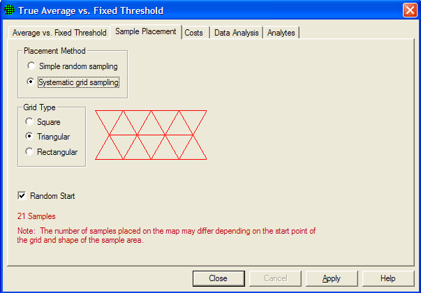
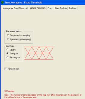
Figure 3.2  Sample Placement for Ordinary Sampling for Selecting Sample Placement Method and Type

• Ordinary sampling - two Sample Placement options are available:

1.       simple random sampling where sampling locations are selected based on random numbers, which are then mapped to the spatial locations, and

2.      systematic grid sampling where sampling locations are selected on a regular pattern (e.g., on a square grid, on a triangular grid, or on a rectangular grid) with the starting location randomly selected. Sampling is done only at the node points of the grid. The grid pattern is selected under Grid Type. Figure 3.2 shows the dialog box for making input selections. You can see an example of the grid pattern selected in red to the right of the Grid Type options. You may specify Random Start or a fixed start for the initial grid point using the check box next to Random Start. Choosing Random Start will generate a new random starting location for the first grid location each time the Apply button is pushed. Once all selections have been made, press Apply.

• stratified sampling - Strata or partitions of an area are made based on a set of criteria, such as homogeneity of contamination. Samples are drawn from each stratum according to a formula that accords more samples to more heterogeneous strata.

• adaptive cluster sampling - An initial n samples are selected randomly. Additional samples are taken at locations surrounding the initial samples where the measurements exceed some threshold value. Several rounds of sampling may be required. Selection probabilities are used to calculate unbiased estimates to compensate for oversampling in some areas.

• sequential sampling - Sequential designs are by their nature iterative, requiring the user to take a few samples (randomly placed) and enter the results into the program before determining whether further sampling is necessary to meet the sampling objectives.

• collaborative sampling - The Collaborative Sampling (CS) design , also called "double sampling", uses two measurement techniques to obtain an estimate of the mean - one technique is the regular analysis method (usually more expensive), the other is inexpensive but less accurate. CS is not a type of sampling design but rather method for selecting which samples are analyzed by which measurement method.

• ranked set sampling - In this two-phased approach, sets of population units are selected and ranked according to some characteristic or feature of the units that is a good indicator of the relative amount of the variable or contaminant of interest that is present. Only the mth ranked unit is chosen from this set and measured. Another set is chosen, and the m-1th ranked unit is chosen and measured. This is repeated until the set with the unit ranked first is chosen and measured. The entire process is repeated for r cycles. Only the m X r samples are used to estimate an overall mean.

• sampling along a swath or transect - Continuous sampling is done along straight lines (swaths) of a certain width using geophysical or radiological sensors capable of continuous detection. Swath patterns can be parallel, square, or rectangular. The goal is to find circular or elliptical targets. This design contains the two elements of traversing the target and detecting the target. VSP application is for unexploded ordnance (UXO) and for detecting radiological hot spots.

• sampling along a boundary - This design places samples along a boundary in segments, combines the samples for a segment, and analyzes each segment to see if contamination has spread beyond the boundary. If contamination has spread, VSP keeps extending the boundary until the sampling goals have been met.

• multiple increment sampling - This design often arises because of the expense associated with analytical tests. A researcher would randomly take n increments and combine them together into r groups for analysis.

• judgment sampling - You simply point and click anywhere in a sampling area. These sampling locations are based on the judgment of the user.

Because judgment sampling is not probability-based, users can bias the sampling results using this method. There is no basis in statistical theory for making confidence statements about conclusions drawn when samples are selected by judgment. However, some problem definitions might call for judgment sampling, such as looking in the most likely spot for evidence of contamination or taking samples at predefined locations. Figure 3.3 shows judgment sampling selected in VSP and six sampling locations selected manually.

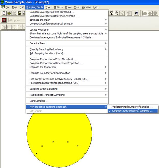
Figure 3.3.  Judgment Sampling in VSP

3.2 DQO Inputs and Sample Size

The inputs needed for VSP's sample-size calculations are decided upon during the DQO process. If you have not gone through the DQO process prior to entering this information, you can enter "best guess" values for each of the inputs and observe the resulting computed sample size. New inputs can be tried until a sample size that is feasible and/or within budget is obtained. This iterative method for using VSP is a valuable "what if" tool with which you can see the effect on sample size (and hence costs) of changing DQO inputs. However, be cautioned that all the DQO elements interact and have special meaning within the context of the problem. To be able to defend the sample size that VSP calculates, you must have a defensible basis for each of the inputs. There is no quick way to generate this defense other than going through Steps 1 through 6 of the DQO process.

The core set of DQO inputs that affect sample size for most of the designs are as follows:

• Null Hypothesis Formulation - The null hypothesis is the working hypothesis or baseline condition of the environment. There must be convincing evidence in the data to declare the baseline condition to be false. VSP uses a default of "Site is Dirty" as the working hypothesis that must be disproved with convincing evidence from the data.

• Type I Error Rate (Alpha) - This is called the false rejection rate in EPA's DQO guidance (EPA 2000a). This is the probability of rejecting a true null hypothesis. For the typical hypothesis test in which we assume the survey unit is dirty (above the action level), alpha is the chance a dirty site with a true mean equal to or greater than the Action Level will be released as clean to the public. In general, alpha is the maximum chance, assuming the DQO inputs are true, that a dirty site will be released as clean.

• Type II Error Rate (Beta) - This is called the false acceptance rate in EPA's DQO guidance. This is the probability of not rejecting (accepting) a false null hypothesis.  For the typical hypothesis test in which we assume the survey unit is dirty, beta is the chance a specific clean site will be condemned as dirty. Specifically, beta is the chance that a clean site with a true mean equal to or less than the lower bound of the gray region will be condemned as dirty. In general, beta is the maximum chance, outside the gray region, that a clean site will be condemned as dirty.

• Width of Gray Region (Delta) - This is the distance from the Action Level to the outer bound of the gray region. For the typical hypothesis test in which we assume the survey unit is dirty, the gray region can be thought of as a range of true means where we are willing to decide that clean sites are dirty with high probability. Typically, these probabilities are 20% to 95%, i.e., from beta to 1 - alpha.  If this region is reduced to a very small range, the sample size grows to be extremely large. Determining a reasonable value for the size of the gray region calls for professional judgment and cost/benefit evaluation.

• Estimated Sampling Standard Deviation - This is an estimate of the standard deviation expected between the multiple samples. This estimate could be obtained from previous studies, previous experience with similar sites and contaminants, or expert opinion. Note that this is the square root of the variance. In one form or another, all the designs require some type of user-input as to the variability of contamination expected in the study area. After all, if the area to be sampled was totally homogeneous, only one sample would be required to completely characterize the area.

Other inputs are required by some of the designs, and other inputs are required for design parameters other than sample size. For example, the stratified designs require the user to specify the desired number of strata and estimates of proportions or standard deviations for each of the stratum. The UXO (unexploded ordinance) modules use Bayesian methods and require the user to input their belief that the study area contains UXO. When simulations are used, as in the post-survey UXO target detection, the user must input assumptions about the distribution of scrap or shrapnel in the target areas.  In the discussions of the designs, we try to give an explanation of each input required of the user.  If you are lost, use the VSP Help functions (See Section 2.7).

Note:  The Help Topics function in VSP provides a description of each of the designs and its related inputs. You can also select the Help button on the toolbar, put the cursor on any of the designs on the menu and a description of the design and its inputs will appear in a Help window. In addition, pressing the Help button at the bottom of each design dialog will bring up a Help window that contains a complete explanation of the design. Finally, on each screen where input is required, highlight an item and press the F1 key for a description of that input item.

The next section contains a discussion of the inputs required by most of the designs available in the current release of VSP. The designs are organized by the Sampling Goal under which they fall.  Not all options for all designs are discussed. Common design features (such as Costs, Historical Samples, MQO) that are found in multiple designs will not be discussed individually in this section but can be found in Section 5.0, Extended Features of VSP. 

3.2.1 Compare Average to a Fixed Threshold

Comparing the average to a fixed threshold is the most common problem confronted by environmental remediation engineers. We present different forms the problem might take and discuss how VSP can be used to address each problem formulation.

We can continue where we left off in Section 2.3.3 with the Millsite.dxf map loaded. We selected a single Sample Area from the site. The Action Level for the contaminant of interest is 6 pCi/g in the top 6 in. of soil. Previous investigations indicate an estimated standard deviation of 2 pCi/g for the contaminant of interest. The null hypothesis for this problem is "Assume Site is Dirty" or H_O: True mean = A.L.

We desire an alpha error rate of 1% and a beta error rate of 1%.  According to EPA (2000a, pp. 6-10), 1% for both alpha and beta are the most stringent limits on decision errors typically encountered for environmental data. We tentatively decide to set the lower bound of the gray region at 5 pCi/g and decide a systematic grid is preferable.

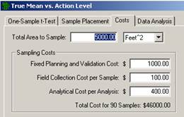
We will use VSP to determine the final width of the gray region and the number of samples required. Assume the fixed cost of planning and validation is $1,000, the field collection cost per sample is $100, and the laboratory analytical cost per sample is $400. We are told to plan on a maximum sampling budget of $20,000.

Case 1:  We assume that the population from which we are sampling is approximately normal or that it is well-behaved enough that the Central Limit Theorem of statistics applies. In other words, the distribution of sample means drawn from the population is approximately normally distributed. We also decided that a systematic pattern for sample locations is better than a random pattern because we want complete coverage of the site.

(a)

(b)                                                              (c)

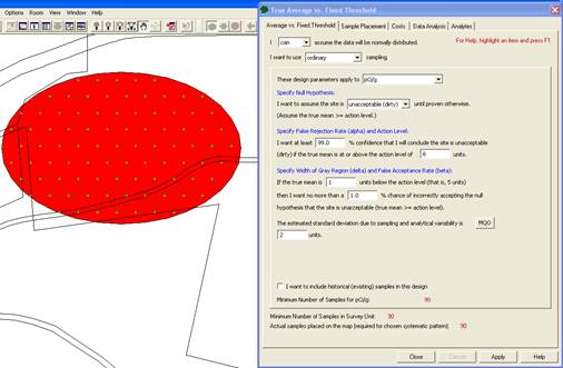
Figure 3.4.  Input Boxes for Case 1 with Original Error Rates

VSP Solution 1: We start by choosing the VSP Sampling Goal option of Compare Average to Fixed Threshold. From the drop-downs, we select that we can assume the data will be normally distributed, and that we want to use ordinary sampling.For Sample Placement, we select Systematic grid sampling. For Grid Type we select Triangular with a Random Start. A grouping of the input dialogs is shown in Figure 3.4.  Note that instead of inputting the alpha error rate directly, it is input as the confidence (100% - alpha%) in correctly accepting the null hypothesis.

We see that for our inputs, using a one-sample t-test will require taking 90 samples at a cost of $46,000. Clearly, we need to relax our error tolerances or request more funding.

For the sake of argument, suppose all the stakeholders agree that an alpha error rate of 5% and a beta error rate of 10% are acceptable. Figure 3.5 reveals that those changes lead to a significant reduction in the sampling cost, now $19,000 for n =36 samples.

Are these new error rates justifiable? Only the specific context of each problem and the professional judgment of those involved can answer that question. What about the assumption that we will be able to use a parametric test, the one-sample t-test? Unless the population from which we are sampling is quite skewed, our new

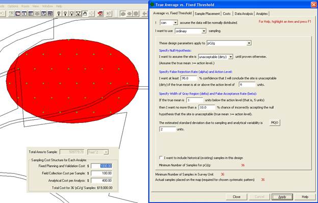
Figure 3.5.  Input Boxes for Case 1 with Increased Error Rates

sample size of n =36 is probably large enough to justify using a parametric test. Of course, once we take the data, we will need to justify our assumptions as pointed out in Guidance for Data Quality Assessment Practical Methods for Data Analysis (EPA 2000b, pp. 3-5).

Case 2:  We now decide that we want to look at designs that may offer us cost savings over the systematic design just presented. We have methods available for collecting and analyzing samples in the field making quick turnaround possible. We want to be efficient and cost-effective and take only enough samples to confidently say whether our site is clean or dirty. After all, if our first several samples exhibit levels of contamination so high that there is no possible scenario for the average to be less than a threshold, why continue to take more samples?  We can make a decision right now that the site needs to be remediated. Sequential designs, and the tests associated with them, take previous sampling results into account and provide rules specifying when sampling can stop and a decision can be made.

VSP Solution 2a:  From VSP's main menu, select the Sampling Goal of Compare Average to a Fixed Threshold.  From the drop-downs, select that we can assume the data will be normally distributed, and that we want to use sequential sampling. The dialog box in Figure 3.6 appears. We begin by entering the DQO parameters for Alpha, Beta, Action Level, etc., which in Figure 3.6 are shown in a sentence structure format.  Next, enter the Number of Samples Per Round, shown here as 3. This parameter indicates how many samples you want to take each time you mobilize into the field.  Each time you press the Apply button, VSP places a pattern of this many sampling locations on the map, except for the first round where at least 10 samples are needed to get an estimate of the standard deviation.

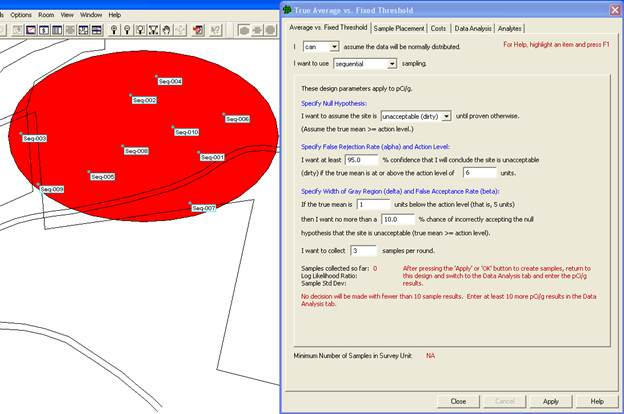
Figure 3.6. Dialog for Sequential Sampling (Standard Deviation Known) and Ten Locations Placed on the Map

In Figure 3.6, we see the results of pressing Apply. Ten locations are placed on the Map labeled "Seq-001, Seq-002, etc."

Once the sample results are available, click on the Data Analysis tab, go to the Data Entry sub-page, and enter the measurement values for those ten samples into the grid on the data input dialog. We enter these values as 5, 8, 6, 7, 5, 4, 8, 4, 7 and 5.  Press the Apply button and in VSP you will see that three more samples have been generated. Return to the Average vs. Fixed Threshold tab.  We now see in Figure 3.7 that the Number of Samples Collected as 10, and that VSP cannot accept or reject the null hypothesis on the basis of these samples and suggests that up to 2 additional samples may be needed to make a decision. (Note that VSP will not accept or reject the null hypothesis with fewer than 10 samples). VSP asks you to take 3 more samples, which are the three new samples placed on the map. 

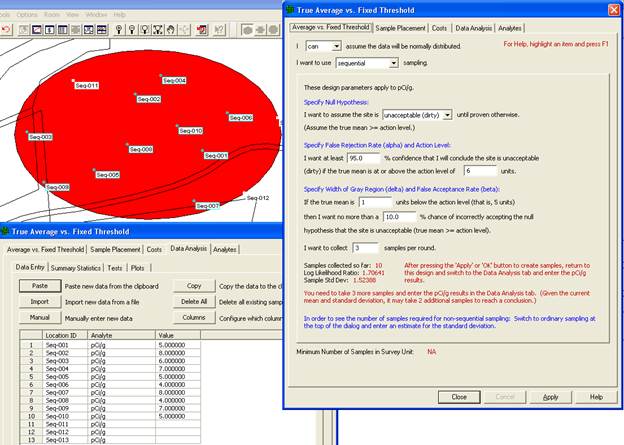
Figure 3.7. Data Input Dialog for Sequential Probability Ratio Test and Results from First Round of Sampling.  Map View is shown in background.

Switching over to the Graph View in Figure 3.8, we can see that in order to accept the null hypothesis that the site is dirty we need to take more than 10 samples. The open circles show the test statistic as the data are collected. The last 3 samples that appear on the graph are the next three samples, which can be entered in the Data Analysis tab's Data Entry sub-page as 6, 7, and 8.  VSP now tells us that we can Accept the Null Hypothesis and conclude the site is dirty.

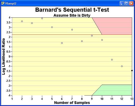
Figure 3.8.  Graph View of Sequential Sampling

VSP Solution 2b.  We have one other option for more cost-efficient sampling - reduce the analytic laboratory costs by taking advantage of measurement equipment that may be less accurate, but is less expensive. (Note that the two methods do not even have to measure the same thing as long as there is a linear correlation between them. For example, the expensive method may measure the concentration of Plutonium metal in soil and the inexpensive method may measure low-energy gamma radiation emitted by Americium in soil. This works because Americium is a daughter product of Plutonium decay). If we can still meet our DQOs (error levels, width of grey region) taking advantage of the less expensive equipment, we will save money.

It works like this: At 'n' field locations selected using simple random sampling or grid sampling, the inexpensive analysis method is used. Then, for some of the 'n' locations, the expensive analysis method is also conducted (n_E). The data from these two analysis methods are used to estimate the mean and the standard error (SE: the standard deviation of the estimated mean). The method of estimating the mean and SE assumes there is a linear relationship between the inexpensive and expensive analysis methods. If the linear correlation between the two methods is sufficiently high (close to 1), and if the cost of the inexpensive analysis method is sufficiently less than that of the expensive analysis method, then Collaborative Sampling (CS) is expected to be more cost effective at estimating the population mean than if the entire measurement budget was spent on obtaining only expensive analysis results at field locations selected using simple random sampling or grid sampling.

If Collaborative Sampling is chosen for the Sampling Goal of Compare Average to a Fixed Threshold the resulting Map View of the applied CS samples on the Millsite.dxf map are all shown in Figure 3.9.

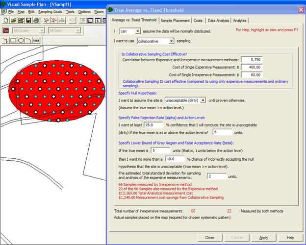
Figure 3.9.     Dialog Box for Collaborative Sampling and Map View of Applied CS Samples

The first set of inputs requested in the Data Input Dialog Box for CS are those needed to determine whether CS sampling is more cost effective than using only expensive measurements and simple random sampling. The first input required is the correlation coefficient between expensive and inexpensive measurements computed on the same set of samples. This is determined from data in prior studies or in a pilot study. The next two inputs are the cost estimates:  the cost per unit of making a single expensive measurement, including the cost of sample collection, handling, preparation and measurement; and the cost per unit of making a single inexpensive measurement, including finding the field location and conducting the inexpensive analysis method.

The next set of inputs comprises the DQOs for the problem. Notice that these are the same inputs we used for Case 1 with increased error rates (see Figure 3.5) when VSP calculated a required sample size of 36. If all those 36 samples were analyzed with the expensive method, the total cost would be 36 x $400=$14,400. However, if we use CS and the same DQOs, VSP calculates we need to take 66 samples measured by the inexpensive method, and 23 of those 66 samples measured by the expensive method. This costs a total of 66 x $60=3960 plus 23 x $400=$9200 for a total of $13,160. This represents a $1,240 cost savings over the $14,400 we were going to spend. And the best part is we can achieve this cost savings and still meet our required error rates (i.e., the stated DQOs). Note: If VSP determined that CS was not cost effective, it would not have computed the two samples n and n_E (66 and 23 samples, respectively) and reported only the number of samples that should be collected and analyzed using only the expensive method (36 samples).

Once we hit the Apply button at the bottom of the Dialog Box, VSP places all 66 samples on the Sample Area on the map. VSP color codes those sample locations where both methods should be used vs. the sample locations where just the inexpensive measurement method should be used. The applied color-coded samples are shown in the Map View insert in Figure 3.10.

We now exit the Dialog Box by clicking on the X in the upper right-hand corner of the display. We take our samples, use the appropriate measurement method, and return to the Data Analysis tab'sData Entry sub-page. The data values can be entered by typing them into this input screen, or by importing the data from a file such as an Excel spreadsheet (see Section 2.4.1 Importing Samples). Figure 3.10 shows the Dialog Box for entering data.

Note that the values we entered result in a Standard Deviation of 2.24 - we estimated 2, and the two sets of sample values have a correlation of .769 - we estimated .75. We are well above the correlation limit of .650 in order for collaborative sampling to be cost effective. If we bring up the Graph View in a second window (View > Graph), we see that VSP has taken the data values we input and plotted the expensive measurements versus the inexpensive measurements. This plot can be used to assess whether the assumption of a linear relationship between the expensive and inexpensive measurements required for the use of CS is reasonable. Note that the calculated Rho=.769 (the correlation coefficient) is listed at the top of the graph. The regression line is the solid red line through the points. The dashed blue line 

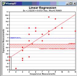
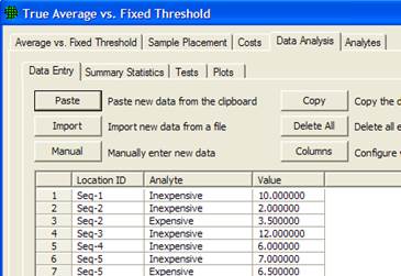
Figure 3.10.      Dialog Box for Entering CS Data Values and Graph View Showing where Data Values Fall on a Linear Regression Line

represents the computed mean (x_cs). The horizontal red line represents the threshold value (Action Level).The bottom edge of the hashed red region represents the computed mean value below which the null hypothesis can be rejected.

VSP reports that based on the data values input, we can Accept the Null Hypothesis: Assume the Site is Dirty.

If we had chosen Simple Random Sampling rather than Systematic Grid Sampling on the Sample Placement tab, all the sample sizes would have been the same. The only difference would have been that the samples would have been placed on the Map in a grid pattern rather than randomly.

Case 3: We do not wish to assume that the population from which we are sampling is approximately normal.

VSP Solution 3a:  The purpose of a MARSSIM sign test is to test a hypothesis involving the true mean or median of a population against an Action Level. Using this test for the mean assumes the distribution of the target population is symmetrical. When the distribution of the target population is symmetrical, the mean and the median are the same. When the distribution is not symmetrical, the Sign test is a true test for the median, and an approximate test for the mean. The appropriate use of the Sign Test for final status surveys is discussed in Multi-Agency Radiation Survey and Site Investigation Manual (MARSSIM) (EPA 1997). This document is currently available at http://www.epa.gov/radiation/marssim/. The input for the MARSSIM Sign Test is shown in Figure 3.11.

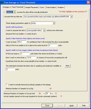
Figure 3.11.   Dialog Box for the MARSSIM Sign Test

VSP Solution 3b: From VSP's main menu, select the Sampling Goal of Compare Average to a Fixed Threshold. From the drop-downs, select that we cannot assume the data will be normally distributed, and that our data are symmetrical (the mean and median are the same). Note that using this test for the mean assumes the distribution of the target population is symmetrical. A grouping of the input dialogs is shown in Figure 3.12.

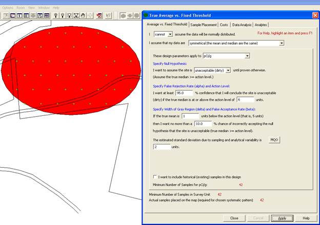
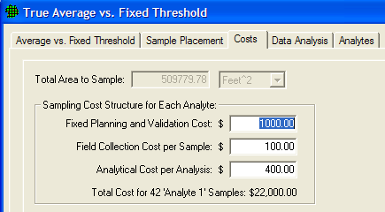
Figure 3.12.    Input Dialog for Wilcoxon Signed Rank Test

For our inputs, and assuming that we will use a nonparametric Wilcoxon Signed Rank test to analyze our data, VSP indicates that we are required to take 42 samples at a cost of $22,000. This is $3,000 more than the previous parametric case, given the same input parameters. Is the choice of a nonparametric test worth the extra $3,000 in sampling costs beyond what was required for the parametric one-sample t-test? VSP does not address that kind of question. Professional judgment is needed.  You must make the decision based on the best available data, the consequences of decision errors, and legal and ethical considerations. If little pre-existing information is available, a pilot study to gain a better understanding of the characteristics of the population may be indicated, since a symmetric distribution of the target population is assumed.

For detailed documentation of the WSR test, please refer to the VSP Help Topic Wilcoxon Signed Rank Test.

3.2.2 Compare Average to Reference Average

We again start with the Millsite.dxf map from Section 2.3.3 with a single Sample Area defined. The Action Level for the contaminant of interest is 5 pCi/g above background in the top 6 in. of soil. Background is found by sampling an appropriate reference area. Previous investigations indicate an estimated standard deviation of 2 pCi/g for the contaminant of interest. The null hypothesis for this problem is "Assume Site is Dirty" or H_O: Difference of True Means = Action Level.  In other words, the parameter of interest for this test is the difference of means, not an individual mean as was the case in the one-sample t-test.

We desire an alpha error rate of 1% and a beta error rate of 1%.  We tentatively decide to set the lower bound of the gray region to 4 pCi/g above background, i.e., a difference of means of 4 pCi/g. Using VSP, we will determine the final width of the gray region and the number of samples required.

Assume that the fixed planning and validation cost is $1,000, the field collection and measurement cost per sample is $100, and the laboratory analytical cost per sample is $0 because we are able to justify the use of field measurements. We are told to plan on a maximum sampling budget of $20,000 for both the Reference Area and the Study Area.

Case 4: We assume that the populations we are sampling are approximately normal or that they are well-­behaved enough so that the Central Limit Theorem of statistics applies. In other words, the distributions of sample means drawn from the two populations are approximately normally distributed. If that is the case, the distribution of the differences also will be approximately normally distributed. We also assume the standard deviations of both populations are approximately equal. In addition, we determine that a systematic grid sampling scheme is preferable.

VSP Solution 4a: We start by choosing from the main menu: Sampling Goals > Compare Average to Reference Average. A grouping of the input dialogs is shown in Figure 3.13.

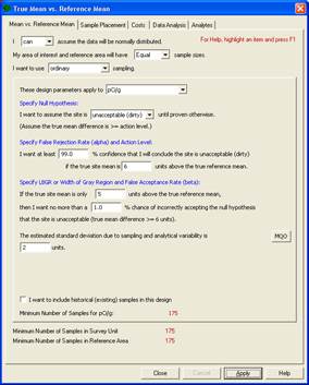
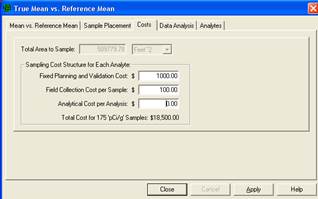
Figure 3.13.   Input Dialogs for Case 4 with Original Error Rates

We see that for our inputs, using a two-sample t-test will require taking 175 field samples in the Sample Area at a cost of $18,500. The sampling cost for the Reference Area also will be $17,500 (assuming the fixed costs will not be incurred a second time). The combined sampling cost of $36,000 is significantly beyond our budget of $20,000. What will be the result if we relax the error rates somewhat?

In Figure 3.14, by increasing both the alpha error rate and the beta error rate to 5%, the sampling cost for one area has decreased to $9,800 based on n =88 field samples. Thus, the new combined cost of $18,600 achieves our goal of no more than $20,000.

Can we justify these larger error rates? Again, only professional judgment using the best information related to the current problem can answer that question.

What about our planned use of a parametric test, the two-sample t-test? A sample size of 88 is large enough that we can probably safely assume the two-sample t-test will meet the assumption of normality for the differences of sample means. We should test this assumption after the data are collected.

What about the assumption of approximately equal standard deviations for the measurements in the Sample and Reference Areas? When we collect the data, we will need to check that assumption. See Guidance for Data Quality Assessment Practical Methods for Data Analysis (EPA 2000b, pp. 3-26) for the use of Satterthwaite's t-test when the standard deviations (or variances) of the two areas are not approximately equal.

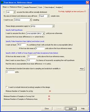
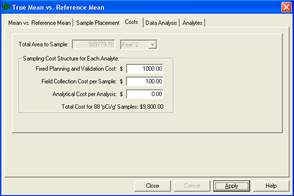
Figure 3.14.   Input Boxes for Case 4 with Increased Error Rates

VSP Solution 4b: Taking the previous example, we now assume that the number of reference samples is fixed at 50, and the standard deviation for the reference samples is expected to be a slightly lower 1.5 pCi/g for the contaminant of interest.  We want to calculate how many field samples to take while still meeting our parameters.  We start by choosing from the main menu: Sampling Goals > Compare Average to Reference and use Unequal sample sizes. The input dialog is shown in Figure 3.15 after entering parameters and clicking Calculate. This module accounts for differences in sample sizes for reference and field samples, and also accounts for differences in standard deviations. VSP has run simulations and estimated that 58 field samples will be needed in addition to the 50 reference samples to achieve the desired alpha and beta levels to run a two-sample t-test.

Case 5:  We now look at the case in which the nonparametric Wilcoxon Rank Sum (WRS) Test is planned for the data analysis phase of the project. VSP offers the MARSSIM version of the WRS Test. If the Sample and Reference population distributions are not symmetric, the WRS method tests the differences in the medians. If one wants to make a statement about the differences between means using the WRS test, it is required that the two distributions be symmetric so that the mean equals the median. 

The Wilcoxon rank sum test is discussed in Guidance for Data Quality Assessment (EPA 2000b, pp. 3-31 - 3-34). The document can be downloaded from the EPA at: http://www.epa.gov/quality/qa_docs.html. It tests a shift in the distributions of two populations. The two distributions are assumed to have the same shape and dispersion, so that one distribution differs by some fixed amount from the other distribution. The user can structure the null and alternative hypothesis to reflect the amount of shift of concern and the direction of the shift.

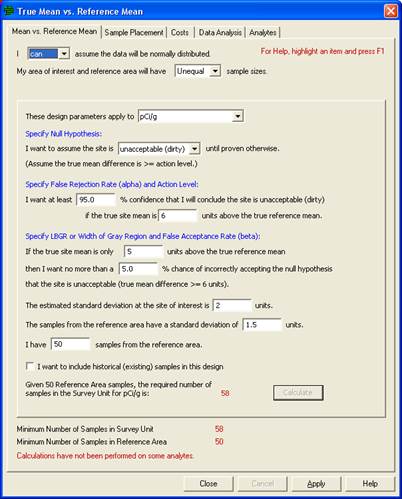
Figure 3.15 Input Dialog for Case 4 with Unequal Sample Sizes and Unequal Standard Deviations

VSP Solution 5: We start by choosing from VSP's main menu Sampling Goals > Compare Average to Reference Average and select that you cannot assume the data are normally distributed. A grouping of the input dialogs is shown in Figure 3.16.

Shown in Figure 3.16, the input dialog for the MARSSIM WRS test allows the user to supply a percent overage to apply to the sample size calculation.  MARSSIM suggests that the number of samples should be increased by at least 20% to account for missing or unusable data and for uncertainty in the calculated values of Sample Size, (EPA 1997, p. 5-29). With the extra 20%, 114 samples are required in both the Sample Area (i.e., Survey Unit or Study Area) and Reference Area.

The cost per area is now $12,400.  The larger sample size of 114 instead of the previous sample size of 88 is probably not justified. However, professional judgment is needed to make the final decision.

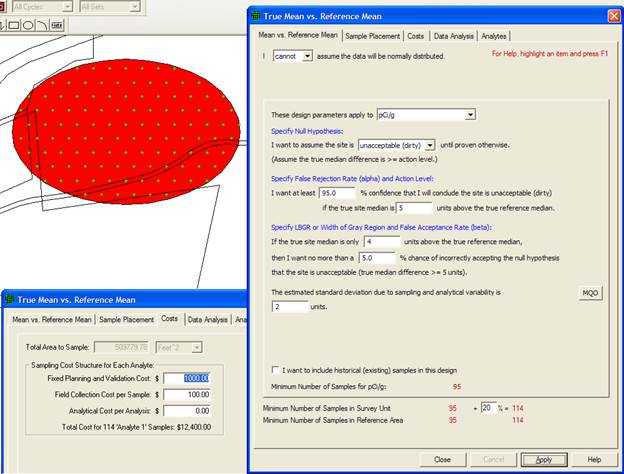
Figure 3.16.   Input Boxes for Case 5 Using Nonparametric Wilcoxon Rank Sum Test

For detailed documentation of the WSR test, please refer to the VSP Help Topic Wilcoxon Signed Rank Test.

The MARSSIM WRS test is used to test whether the true median in a Survey Unit population is greater than the true median in a Reference Area population. The test compares medians of the two populations because the WRS is based on ranks rather than the measurements themselves. Note that if both the Survey Unit and Reference Area populations are symmetric, then the median and mean of each distribution are identical.  In that special case the MARSSIM WRS test is comparing means. The assumption of symmetry and the appropriate use of the WRS test for final status surveys is discussed in Multi-Agency Radiation Survey and Site Investigation Manual (MARSSIM) (EPA 2000). This document is currently available at:  http://www.epa.gov/radiation/marssim/.

Case 6:  Next, assume that the population from which we will be sampling is non-normal but symmetric and we again desire to use a nonparametric Wilcoxon rank sum test. However, we are limited to a total sampling budget for both areas of $10,000. By using VSP iteratively, we will adjust the various DQO input parameters and try to discover a sampling plan that will meet the new goals.

VSP Solution 6: Figure 3.17 shows that with an alpha of 5%, a beta of 12.5%, and a lower bound of the gray region of 3.5, the number of samples per area drops to 39. With a sampling cost of $3,900 for each sampling area, and assuming the fixed costs of $1,000 will only occur once, we now have a combined cost of $8,800 and thus meet our goal of $10,000.

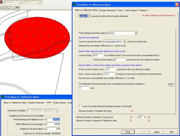
Figure 3.17.   Input Boxes for Case 6 Using Nonparametric Wilcoxon Rank Sum Test

Will relaxing the error tolerances and increasing the width of the gray region to meet the requirements of the smaller sampling budget be acceptable to all stakeholders in the DQO process? Again, it depends on the objectives and judgment of those involved in the process.

Case 7: Suppose our combined sampling budget is reduced to $5,000. Can VSP provide a sampling design that meets that goal?

VSP Solution 7: Figure 3.18 shows a design with just 15 samples per sampling area that meets the new sparse budget. We reduced the combined sampling cost, now $5,000, by increasing the width of the gray region to 2.35 pCi/g (lower bound of the gray region is 2.65 pCi/g) and by increasing the beta level to 0.20 (20%).

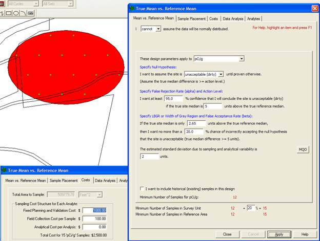
Figure 3.18.   Input Boxes for Case 7 Using Nonparametric Wilcoxon Rank Sum Test

There are definite consequences of reducing sampling requirements to fit a budget. The consequences could include a greater chance of concluding that a dirty site is clean or a clean site is dirty. There is also a larger area of the gray region where you say you will not control (i.e., limit) the false acceptance error rate.

Is it justifiable to keep reducing the sampling budget in the above manner? Again, the answer depends on the specific problem. VSP, like most software, suffers from GIGO - Garbage In, Garbage Out. However, a responsible DQO process can provide valid information to VSP that overcomes GIGO and lets VSP help solve the current problem in an efficient manner.

Case 8: Now we assume we have seriously underestimated the standard deviation. Suppose that instead of 2 pCi/g, it is really 4 pCi/g. Now how many samples should we be taking?

VSP Solution 8: Figure 3.19 shows the new sample size has jumped to 53, almost a four-fold increase over the 14 samples used in VSP Solution 7. For many sample-size equations, the number of required samples is proportional to the square of the standard deviation, i.e., the variance. Thus, an underestimate of the standard deviation can lead to a serious underestimate of the required sample size.

If we seriously underestimate the standard deviation of the measurements, what will be the practical implications of taking too few samples? Remember that we have as a null hypothesis "Site is Dirty." If the site is really clean, taking too few measurements means we may have little chance of rejecting the null hypothesis of a dirty site. This is because we simply do not collect enough evidence to "make the case," statistically speaking.

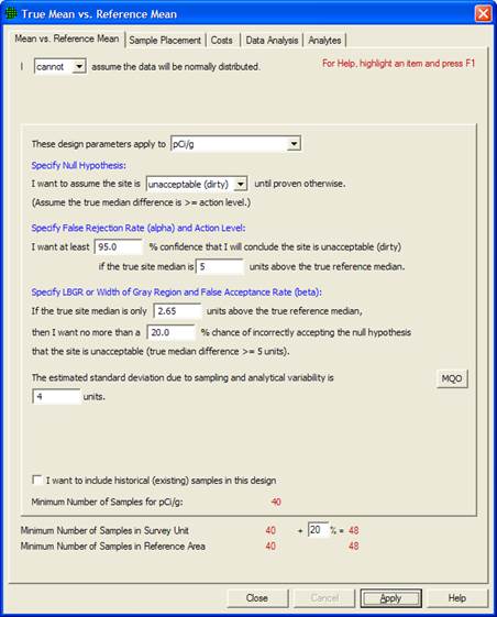
Figure 3.19.   Input Boxes for Case 8 with Larger Standard Deviation

3.2.3 Estimate the Mean

When the Sampling Goal is to Estimate the Mean > Data not required to be normally distributed, three design options are offered in VSP. None of the three requires the assumption of normality as the underlying distribution of units in the population. The options are:

• Stratified sampling

• Ranked set sampling

• Collaborative sampling

For additional information on estimating the mean, please refer to the VSP Help Topic Estimate the Mean menu commands.

3.2.3.1 Stratified Sampling

In Figure 3.20, we see the dialog box for entering parameters for stratified sampling. Prior to running VSP to calculate sample sizes for the strata, the user must have pre-existing information to divide the site into non-overlapping strata that are expected to be more homogeneous internally than for the entire site (i.e., all strata). They must be homogeneous in the variable of interest for which we want to calculate a mean. The strata are the individual user-selected Sample Areas and can be seen using Map View.

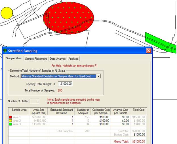
Figure 3.20.   Dialog Box for Stratified Sampling for Estimating a Mean

With the Sample Areas selected (VSP shows total number of areas in Numbers of Strata), the dialog shows the initial values VSP assigns to the various inputs. The number of potential samples in each stratum is initially set at the number of 1-square-foot (or whatever units are used) units available to be sampled or approximately the area of the Sample Area (shown when the area is first selected). If the sample support is not a 1-square-foot volume, the user should change this to the correct value. The initial standard deviation between individual units in the stratum is assigned the value 1. It is in the same units as the mean. This is a critical value in the sample size calculation, so the user should make sure this is a good estimate. The sampling and measurement costs per sample in each stratum and the fixed costs are input in dollars. After entering the values for stratum 1, the user selects the next stratum from the drop-down list under Stratum #.

VSP allows simple random sampling or systematic within the strata. This is selected within the Sample Placement tab (Figure 3.21).

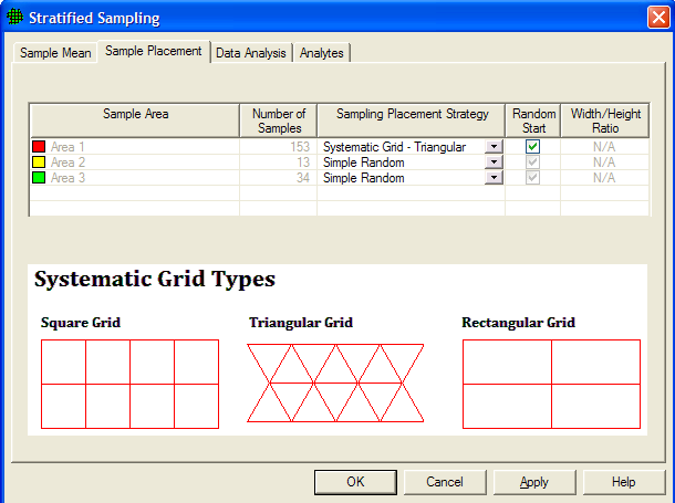
Figure 3.21.      Sample Placement for Stratified Sampling for Estimating a Mean

The other inputs required by VSP pertain to the method the user wants to use for determining 1) the total number or samples in all strata and 2) the allocation of samples to strata.  Methods are selected from the drop-down lists. VSP Help offers some insight into why one method might be selected over another, but the user should use the DQO process to flush out the site-specific conditions and project goals that will determine these inputs. Different inputs are required depending on which method is selected for determining the total number of samples. After you press Apply, the dialog shows in red the total number of samples and the number of samples in each stratum (use the pull-down Stratum # to switch between strata). You can see the placement of samples within strata by going to Map View.

For detailed documentation on Stratified Sampling, please refer to the VSP Help Topic Stratified Sampling for Estimating a Mean.

3.2.3.2 Ranked Set Sampling

Ranked set sampling (RSS) is the second option for the Sampling Goal: Estimate the Mean > Data not required to be normally distributed. The number of inputs required for RSS is the most of any of the designs available in VSP. However, RSS may offer significant cost savings, making the effort to evaluate the design worthwhile. The VSP Help, the VSP technical report (Gilbert et al. 2002), and EPA (2002, pp. 79-111) are good resources for understanding what is required and how VSP uses the input to create a sampling design.

A simple example given here will explain the various input options. The user should have gone through the DQO process prior to encountering this screen because it provides a basis for inputs.

Under the tab Ranked Set Sampling, the first set of inputs deals with whether this design has any cost advantages over simple random sampling or systematic sampling where every unit that is sampled is measured and analyzed.

We select Symmetric for the distribution of lab data, thus telling VSP we think the lab data is not skewed so VSP should use a balanced design. A balanced design has the same number of cycles, say r =4, sampled for each of the say m =3 ranks (in this case the set size is 3). That is, a sample is collected at each of the four locations expected to have a relatively small value of the variable of interest, as well as at the four locations expected to have a mid-range value, and at four locations expected to have a relatively large value.  An unbalanced design has more samples collected at locations expected to have large values. EPA says that a balanced design should be used if the underlying distribution of the population is symmetric (EPA 2002, p. 86).

We select Professional Judgment as the ranking method. We choose a set size of 3 from the pull-down menu. The set size we select is based on practical constraints on either our judgment or the field screening equipment available.

Note: VSP uses set size to calculate the factor by which the cost of ranking field locations must be less than lab measurement costs in order to make RSS cost-effective.

The next set of inputs required for RSS is information required to calculate the number of samples needed for simple random sampling. This value, along with cost information, is used to calculate the number of cycles, r. We say we want a one-sided confidence interval (we want a tight upper bound on the mean and are not concerned about underestimates of the sample mean), we want that interval to contain 95% of the possible estimates we might make of the sample mean, we want that interval width to be no greater than 1 (in units of how the sample mean is measured), and we estimate the standard deviation between individual units in the population to be 3 (in units of how the sample mean is measured). VSP tells us that if we have these specifications, we would need 27 samples if we were to take them randomly and measure each one in an analytical lab.

The box in the lower right corner of this dialog gives us VSP's recommendations for our RSS design: we need to rank a total of 45 locations. However, we need to send only 15 of those off to a lab for accurate measurement. This is quite a savings over the 27 required for simple random sampling. There will be r =5 cycles required.

Note: If we had chosen an unbalanced design, VSP would tell us how many times the top ranked location needed to be sampled per cycle. Also, the inputs for the confidence interval would change slightly for the unbalanced design.

All costs (fixed, field collection per sample, analytical cost for sending a sample to the lab, and ranking cost per location) are entered on the dialog box that appears when the Cost tab is selected. In Figure 3.22, we see the two dialog boxes for RSS.

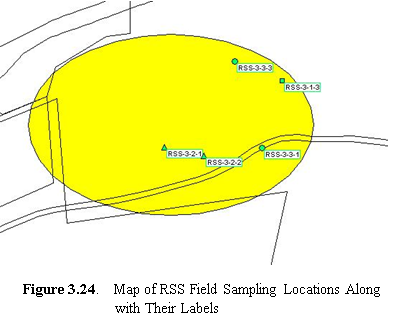
Once we press Apply, the RSS toolbar appears on our screen. The RSS toolbar lets us explore the locations to be ranked and the locations to be sampled and measured under Map View.  VSP produces sample markers on the map that have different shapes and colors. The color of the marker indicates its cycle. The cycle colors start at red and go through the spectrum to violet. Selecting one of the cycles on the pull-down menu displays only the field locations for that cycle. In Figure 3.23, all the green field locations for Cycle 3 are shown. The shape of the marker indicates its set. Field sample locations for the first set are

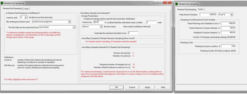
Figure 3.22.   Dialog Boxes for Ranked Set Sampling Design

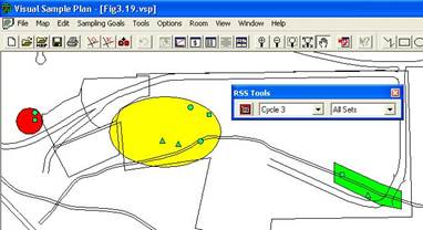
Figure 3.23.   Map of RSS Field Sample Locations for All Sets in Cycle 3, Along with RSS Toolbar

marked with squares, locations for the second set are marked with triangles, and so on. We show All Sets in Figure 3.23. For unbalanced designs, the top set is sampled several times, so a number accompanies those markers. Our example is for a balanced design so we do not see numbers.

Ranked set field sampling locations are generated with a label having the following format: RSS-c-s-i

where  c =  the cycle number

s =  the set number (the unbalanced design for this number is also incremented for each iteration of the top set)

I =  a unique identifier within the set.

Use View > Labels > Labels on the main menu or the AB button on the main toolbar (button also on the RSS toolbar) to show or hide the labels for the field sample locations. Figure 3.24 shows the labels on the map for field sample locations associated with Cycle 3, All Sets.

For detailed documentation on Ranked Set Sampling, please refer to the VSP Help Topic Ranked Set Sampling Design for Estimating a Mean.

3.2.3.3 Collaborative Sampling for Estimating the Mean

The third design we discuss for a cost-effective option for estimating the mean when normality cannot be assumed is Collaborative Sampling (CS) - sometimes called Double Sampling. This design is applicable where two or more techniques are available for measuring the amount of pollutant in an environmental sample, for example a field method (inexpensive, less accurate) and a fixed lab method (expensive, more accurate). The approach is to use both techniques on a small number of samples, and supplement this information with a larger of number of samples measured only by the more expensive method. This approach will be cost-effective if the linear correlation between measurements obtained by both techniques on the same samples is sufficiently near 1 and if the less accurate method is substantially less costly than the more accurate method

Collaborative Sampling works like this:  At n field locations selected using simple random sampling or grid sampling, the inexpensive analysis method is used. Then, for each of n_E of the n locations, the expensive analysis method is also conducted. The data from these two analysis methods are used to estimate the mean and the standard error (SE: the standard deviation of the estimated mean). The method of estimating the mean and SE assumes there is a linear relationship between the inexpensive and expensive analysis methods.

VSP has an extensive discussion of CS in the Help. CS is also discussed in Gilbert (1987), Chapter 9, where you can find an actual Case Study using CS.  In Figure 3.25 we show the input screen for Collaborative Sampling.

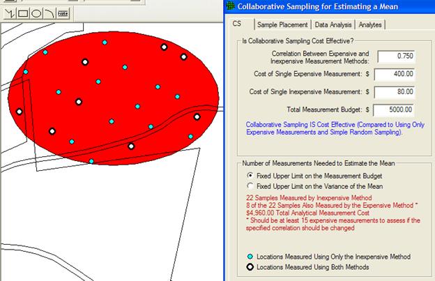
Figure 3.25.   Input Dialog Box for Collaborative Sampling for Estimating the Mean

For this example, we applied CS samples to an area on the Millsite map. After inputting the costs of each measurement technique, the total budget, and an estimate of the correlation between the two methods, VSP informs you whether or not CS is cost effective. For the vales we input, we see that it is cost effective. Then VSP uses the formulas discussed in the On-Line Help and the Report view to calculate two sample sizes, n (22), and n_E (8). There are two options for optimizing the values of n and n_E that the VSP user must select from:

• estimate the mean with the lowest possible standard error (SE: the standard deviation of the estimated mean) under the restriction that there is a limit on the total budget, or

• estimate the mean under the restriction that the variance of the estimated mean (square of the SE) does not exceed the variance of the mean that would be achieved if the entire budget were devoted to doing only expensive analyses.

We select the first option. VSP calculates that we need to take 22 samples and measure them with the inexpensive method, 8 of which are also measured using the more expensive methods. However, we get a warning message that we should be taking at least 15 measurements where we use both methods in order for VSP to assess whether our initial estimate of a 0.75 linear correlation coefficient is correct. Note that after we hit the Apply button, we see the sampling locations placed on the Sample Area we selected (Millsite.dxf used for this example). 

As with Collaborative Sampling for Hypothesis Testing discussed in Section 3.2.1, VSP allows us to input the results of the sampling to verify that the computed correlation coefficient is close to the estimated correlation coefficient used to calculate the sample sizes. Data Results are input in the dialog box that appears after selecting the Data Analysis tab and the Data Entry sub-page. VSP calculates the estimated mean and standard deviation of the estimated mean once the data values are input.

For detailed documentation on Collaborative Sampling, please refer to the VSP Help Topic Collaborative Sampling for Estimating a Mean.

3.2.3.4 Adaptive Cluster Sampling

Adaptive cluster sampling is appropriate if we can assume the target population is normally distributed: Sampling Goal > Estimate the Mean > Can assume data will be normally distributed > Adaptive Cluster Sampling. Because adaptive designs change as the results of previous sampling become available, adaptive cluster sampling is one of the two VSP designs that require the user to enter sample values while planning a sampling plan. (The other design that requires entering results of previous sampling is sequential sampling; see Section 3.2.1). The VSP Help, the VSP technical report (Gilbert et al. 2002), and the EPA (2001, pp. 105-112) are good resources for understanding what is required and how VSP uses the input to create a sampling design. A simple example here will explain the various input options. The user should have gone through the DQO process prior to encountering this screen because it provides a basis for inputs.

The screen for entering values in the dialog box is displayed by selecting the tab Number of Initial Samples. Adaptive cluster sampling begins by using a probability-based design such as simple random sampling to select an initial set of field units (locations) to sample. To determine this initial sample number, either a one-sided or two-sided confidence interval is selected. We select One-sided Confidence Interval and enter that we want a 95% confidence that the true value of the mean is within this interval. We want an interval width of at least 1 and we estimate the standard deviation between individual units in the population to be 2 (units of measure for interval width and standard deviation is same as that of individual sample values). VSP returns a value of 13 as the minimum number of initial samples we must take in the Sample Area. In Figure 3.26, we can see the 13 initial samples as yellow squares on the map.

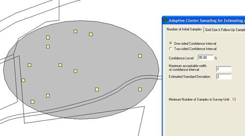
Figure 3.26. Map of Sample Area with Initial Samples for Adaptive Cluster Sampling Shown as Yellow Squares, Along with Dialog Box

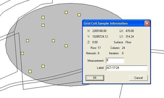
Figure 3.27. Dialog Input Box for Entering Sample Measurement Values and Labels for Initial Samples in Adaptive Cluster Sampling

Select tab Grid Size & Follow-Up Samples on the Adaptive Cluster for Estimating a Mean dialog box. Enter the desired Grid Size for Samples, shown here as 20 ft, and an upper threshold measure­ment value that, if exceeded, triggers additional sampling. We chose 10 as the threshold. We have a choice of how to expand sampling once the threshold is exceeded: 4 nearest neighbors or 8 nearest neighbors. We choose 4. The dialog box is shown as the insert in Figure 3.28. The grid units can be orientated at different angles by selecting Edit > Sample Areas > Set Grid Angle and Edit > Sample Areas > Reset Grid Angle from the main menu.

The user now enters the analytical meas­urement results for the initial 13 sampling units. (Adaptive cluster sampling is most useful when quick turnaround of analytical results is possible, e.g., use of field measurement technology.) Place the mouse directly over each sample and right-click. An input box appears as shown in Figure 3.27. Enter a measurement value (shown here as 8) and, if desired, a label (shown here as AC1-25-62).  Press OK. Enter another sample value and continue until all 13 sample values have been entered.

Once Measurement values have been entered, the yellow squares turn to either green, indicating the sample did not exceed the threshold, or red, indicating the sample exceeded the threshold. The red samples are surrounded with additional yellow squares that now must be sampled. This process continues until there are no more yellow grid cells. In Figure 3.29, we see examples of green, single yellow, red surrounded by yellow, and red surrounded by green. Sampling and measurement continues until all the initial samples are green or red and all the added samples are green or red.

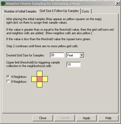
Figure 3.28.   Dialog Input Box for Entering Grid Size and Follow-up Samples

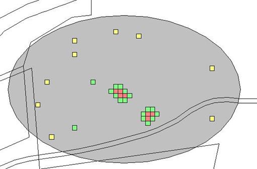
Figure 3.29. Examples of Combinations of Initial and Follow-up Samples from Adaptive Cluster Sampling

Costs are entered using the Cost tab on the dialog box. The Report for adaptive cluster sampling shows the total cost for all the initial samples plus follow-up samples and provides an (unbiased) estimate of the mean and its standard error. Refer to VSP's Help for a complete discussion of adaptive cluster sampling.

For detailed documentation on Adaptive Cluster Sampling, please refer to the VSP Help Topic Adaptive Cluster Sampling for Estimating a Mean.

3.2.4 Construct Confidence Interval on Mean

If the VSP user wants a confidence interval on the true value of the mean, not just a point estimate of the mean as calculated in Section 3.2.3, the user selects Sampling Goal > Construct Confidence Interval on the Mean. When the data can be assumed to be normally distributed, the user can choose Ordinary Sampling, Collaborative Sampling, or Multiple Increment Sampling.

For Ordinary Sampling, four DQO inputs are required:

• whether a one- or two-sided interval is desired,

• the confidence you want to have that the interval does indeed contain the true value of the mean,

• the maximum acceptable half-width of confidence interval, and

• an estimate of the standard deviation between individual units of the popula­tion.

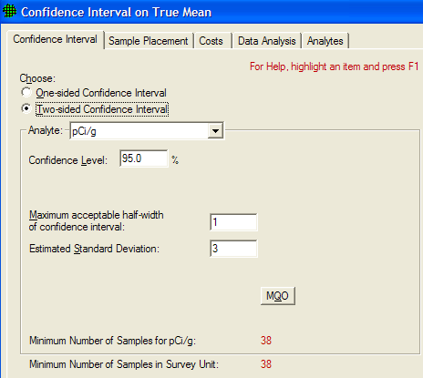
Figure 3.30. Dialog Input Box for Calculating a Confidence Interval on the Mean using Ordinary Sampling

The two-sided confidence interval, smaller interval width sizes, and larger variation generally require more samples. In Figure 3.30, we see an example of the design dialog for the Confidence Interval on the Mean sampling goal for Ordinary Sampling, along with the recommended sample size of 38 that VSP calculated.

If the user has more than one type of sample measurement method available, Collaborative Sampling should be explored to see if cost savings are available. Though not shown here, the inputs for Collaborative Sampling for Confidence Interval are similar to those in Figure 3.29, with the added cost inputs required to determine if Collaborative Sampling is cost effective (see discussion of Collaborative Sampling in Section 3.2.3.3). Note that under the sampling goal of Construct Confidence Interval on the Mean, Collaborative Sampling is put under the assumption of "normality", while for the sampling goal of Estimate the Mean, Collaborative Sampling is put under the assumption of "Data not required to be normally distributed." This is because for Estimating the Mean, the calculation of sample size n is based on restrictions on the budget or restrictions on the variance which make no distributional assumptions; while for Construct Confidence Interval on the Mean, the calculation of n is based on percentiles of the standard normal distribution.

If samples will be combined for analysis, then Multiple Increment Sampling can be selected. This method has additional inputs concerning between increment and within increment standard deviations, and the number of samples being combined. 

If we cannot assume data will be normally distributed, VSP computes a non-parametric confidence interval. The user specifies a one or two-sided confidence interval, and the percent confidence they wish to attain to be within a specified number of percentiles of the true mean (Figure 3.31).

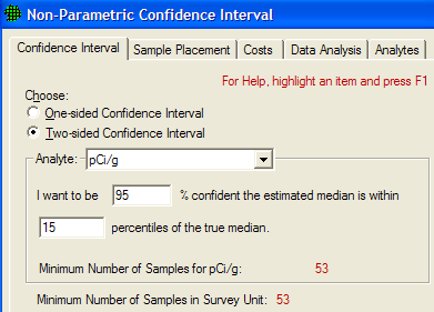
Figure 3.31. Dialog Input Box for Calculating a Non-Parametric Confidence Interval on the Mean using Ordinary Sampling

For detailed documentation on how to construct confidence interval on mean, please refer to the VSP Help Topic Construct Confidence Interval on Mean menu commands.

3.2.5 Compare Proportion to Fixed Threshold

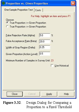
For comparing a proportion to a threshold (i.e., a given proportion), the designs available in VSP do not require the normality assumption. A one-sample proportion test is the basis for calculating sample size. The inputs required to calculate sample size are shown in the design dialog in Figure 3.32. The DQO inputs are similar to those for comparing an average to a fixed threshold, but since the variable of interest is a proportion (percentage of values that meet a certain criterion or fall into a certain class) rather a measurement, the action level is stated as a value from 0.01 to 0.99. Based on the inputs shown in Figure 3.32, VSP calculates that a sample size of 23 is required.

For detailed documentation on compare proportion to fixed threshold, please refer to the VSP Help Topic Compare Proportion to Fixed Threshold.

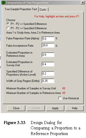
3.2.6 Compare Proportion to Reference Proportion

VSP formulates this problem as an environmental cleanup problem in which we have the proportion of contamination within a survey unit (Population 1) and we want to see if the difference between it and a reference area (Population 2) is greater (or less than) a specified difference. This specified difference becomes the action level. If we select the first formulation of the problem (P1 - P2 = specified difference), we must enter a lower bound for the gray region. If we select the second formulation (P1 - P2 = specified difference), we must enter an upper bound for the gray region. We must also enter our best guess of what we think the proportion of contamination is in both the survey unit and the reference unit. These two values are required to estimate the standard deviation of the proportions, which are then used as inputs to the sample size formula.

Note that if the proportion of interest is the proportion of positive units in the environment, say the proportion of one-acre lots within a development area that have trees, then we need to select the null hypothesis that affords us the greatest protection against a false acceptance. In Figure 3.33, we see an example of the design dialog for this sampling goal. VSP calculates that we need 49 samples in the survey unit and 49 samples in the reference area for this set of inputs.

If no previous information is available on which to estimate the proportions in the survey unit or reference area, use 0.5 because at that value the sample sizes are the largest (i.e., the most conservative).

3.2.7 Estimate the Proportion

Similar to the designs available for estimating the mean, VSP offers stratified sampling for the sampling goal of estimating the proportion because a stratified design may be more efficient than either simple random sampling or systematic sampling. Designs and sample size formulas for a simple random selection of samples are not in the current release of VSP but can be found in standard statistics textbooks.

3.2.8 Locating a Hot Spot

There will be occasions when it is necessary to determine with a specified high probability that no hot spots of a specified size and shape exist in the study area. A hot spot is a local contiguous area that has concentrations that exceed a threshold value.  Initially, the conceptual site model should be developed and used to hypothesize where hot spots are most likely to be present. If no hot spots are found by sampling at the most likely locations, then VSP can be used to set up a systematic square, rectangular or triangular sampling grid to search for hot spots.  Samples or measurements are made at the nodes of the systematic grid. The VSP user specifies the size and shape of the hot spot of concern, the available funds for collecting and measuring samples, and the desired probability of finding a hot spot of critical size and shape. Either circular or elliptical hot spots can be specified.

The VSP user can direct VSP to compute one or more of the following outputs:

• The number and spacing of samples on the systematic sampling grid that are required to achieve a specified high probability that at least one of the samples will fall on a circular or elliptical hotspot of the specified size.

• The probability that at least one of the samples collected at the nodes of the specified systematic sampling grid will fall on a circular or elliptical hot spot of specified size.

• The smallest size circular or elliptical hot spot that will be detected with specified high probability by sampling at the nodes of the systematic sampling grid.

The basic structure for these problems is that there are three variables (grid spacing, size of hot spot, and probability of hitting a hot spot). You can fix any two of them and solve for the remaining variable.

The other unique feature of the hot spot problem is that there is only one type of error-the false negative or alpha error. VSP asks for only one probability for some formulations of the problem-the limit you want to place on missing a hot spot if it does indeed exist. The other error, saying a hot spot exists when it doesn't, cannot occur because we assume that if we do get a "hit" at one of the nodes, it is unambiguous (we hit a hot spot). We define hot spots as having a certain fixed size and shape, i.e., no amorphous, contouring hot spots are allowed. The hot spot problem is not a test of a hypothesis. Rather, it is a geometry problem of how likely it is that you could have a hot spot of a certain size and shape fitted within a grid, and none of the nodes fall upon the hot spot.

All the input dialog boxes for the Hot Spot problem will not be shown in this user's manual.  VSP's Help and the textbook Statistical Methods for Environmental Pollution Monitoring (Gilbert 1987) are good resources for a complete discussion of the Hot Spot problem.  We demonstrate a common formulation of the problem-find the minimum number of samples to find a hot spot of a certain size, with specified confidence of hitting the hot spot. 

Problem Statement: A site has one Sample Area of one acre (43,560 square feet). We wish to determine the triangular grid spacing necessary to locate a potential circular pocket of contamination with a radius of 15 feet. We desire the probability of detecting such a hot spot, if it exists, to be at least 95%. The fixed planning and validation cost is $1,000. The field collection cost per sample is $50, and the laboratory analytical cost per sample is $100. Assume that the budget will be provided to support the sampling design determined from these requirements.

Case 9: We assume that the assumptions listed in Gilbert (1987, p. 119) are valid for our problem. We specify a hit probability of 95%, a shape of 1.0 (circular), and a radius (Length of Semi-Major Axis) of 15 feet. We will let VSP calculate the length of the side of the equilateral triangular grid needed for these inputs.

VSP Solution 9: First, open the file OneAcre.vsp using VSP Main Menu option File > Open Project. This is a VSP-formatted project file and it contains a previously defined Sample Area of the entire acre. Next, from the VSP Main Menu select Sampling Goals > Locating a Hot Spot > Assume no false negative errors. A grouping of the input dialogs for the four tabs: Locating Hot Spot, Grid, Hot Spot, and Costs are shown in Figure 3.34.

The recommended length of grid side is shown in the dialog box for Locating a Hot Spot, Solve for Grid Spacing. It is about 28.98 feet or, rounding up, a 30-foot triangular grid.

Note: For this set of inputs, VSP will always give the length of the triangular grid as 28.98 feet. The Calculated total number of samples in the Report View is always 60 for this set of inputs. However, the Number of samples on the map changes as you repeatedly press the Apply button. This occurs whenever the Random Start check box in the dialog box tabbed Find Grid is checked. Because the starting point of the grid is random, the way in which the grid will fit inside the Study Area can change with each new random-start location. More or fewer sampling locations will occur with the same grid size, depending on how the sampling locations fall with respect to the Sample Area's outside edges.

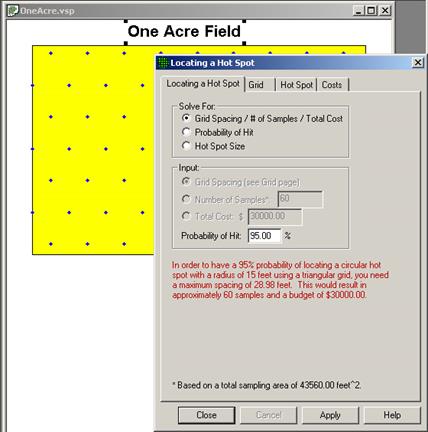
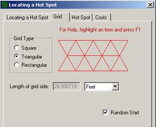
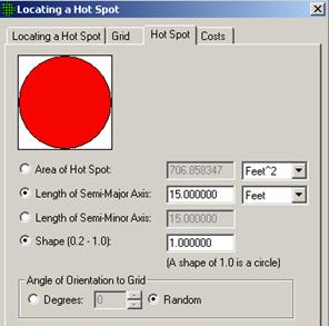
Figure 3.34.   Input Boxes for Case 9 for Locating a Hot Spot

The input dialog boxes and report for the hot spot problem have some unique features:

• Placing the cursor in the Length of Semi-Major Axis on the Hot Spot tab and right-clicking displays a black line on the picture of the circle for the radius.

• Shape controls how "circular" the hot spot is. Smaller values (0.2) result in a more elliptical shape; 1.0 is a perfect circle.

• The user can specify the Area of the hot spot or the Length of the Semi-Major Axis. Both fields have pull-down menus for selecting the unit of measurement.

• The Report provides additional information on the design such as the number of samples (both "on the map" and "calculated") and grid area.

The Hot Spot Sampling Goal takes into account the Total Area to Sample (see this field on the Cost tab) when calculating total number of samples. Many of the other designs use the standard deviation to control sample size.

Selecting Sampling Goals > Locating a Hot Spot > Account for false negative errors provides an option for entering a false negative rate for each sample (the probability each contaminated sample will not be detected). For this option, only circular (Shape=1) hot spots may be used.

Selecting Sampling Goals > Locating a Hot Spot > Using existing locations provides an option for adding additional sampling locations to some previously collected to minimize the locations where circular hot spots may exist on a site.

For further information on locating hotspots, please refer to the VSP Help Topic Detecting Hot Spots.

3.2.9 Find UXO Target Areas

This Sampling Goal originated from specific unexploded ordinance (UXO) problems faced by the Department of Defense. The sampling designs the VSP developers came up with to address these problems are somewhat specialized.  UXO methods are covered in Chapter 7.

3.2.10 Access Degree of Confidence in UXO Presence

This Sampling Goal also originates from UXO Problems, and is covered in Chapter 7.

3.2.11 Non-statistical Sampling Approach

VSP allows the user to directly place samples in a Sample Area without going through the Sampling Goals and the DQO Process. If the user has a pre-determined number of samples, possibly obtained from a prior DQO study, VSP allows the user to input a sample size and place the samples within the Sample Area using either a random design or a systematic design. Menu selection Sampling Goals > Non-Statistical Sampling Approach > Predetermined Number of Samples brings up a simple dialog box where the user can input any value for Number of Samples, and by hitting the Apply button, the samples are placed in the Sample Area according to the design specified (random or systematic).

 VSP allows the user to manually place samples on a Map within a selected Sample Area by selecting Sampling Goals > Non-Statistical Sampling Approach > Judgment (authoritative) Sampling. This option is available only if View > Map is selected and a Sample Area is defined. Judgment Sampling is a toggle switch. When it is turned on, any time the user clicks on the map, a sample marker is placed at that location. Judgment samples can be added to a blank Map or to an existing design. The Type is "Manual" (see View > Coordinates). Manual samples may also be added by typing the coordinates (x, y) on the keyboard.

In Figure 3.35, 6 samples have manually been added using Judgment Sampling.

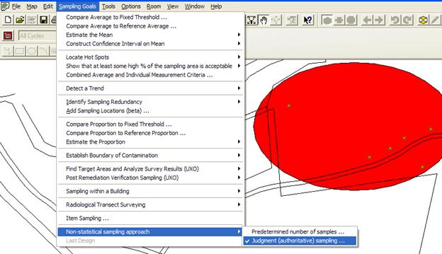
Figure 3.35.   Judgment Sampling with Six Sampling Locations Added Manually

For detailed documentation on non-statistical sampling approaches, please refer to the VSP Help Topic Non-statistical Sampling Approach menu commands.

3.2.12 Establish Boundary of Contamination

Finding the boundary of contamination is a problem faced by Department of Defense remediation managers. Training ranges or areas where the soil is known to contain explosive residues (or other contaminants of concern) may have boundaries that completely or partially enclose the contaminated area. Sampling is required to determine whether contamination has breached a known boundary line and if so, determine the correct boundary line. VSP has a special module for this sampling problem. The problem and the VSP solution are described in Visual Sample Plan User's Guide for Establishing the Boundary of Contamination, R.O. Gilbert, et al, PNWD-3580, 2005, which can be downloaded from the VSP web site http://vsp.pnl.gov. In this User's Guide we will provide a summary description of the VSP boundary module.

The VSP sampling design for this problem involves taking a representative sample (called a multiple increment or MI) for each segment along the known, user-input boundary. If the one or more samples show contamination, extend or "bump out" the boundary, and take more samples. The boundary continues to be bumped out until all samples taken along the new boundary line are "clean". 

In Sections 2.3.1.1 and 2.3.1.2 we described how to define enclosing and partial boundaries in VSP using Edit > Sample Areas > Define New Sample Area, and Edit > Sample Areas > Define New Open-Type Sample Area, respectively. VSP determines the number of segments using the length of the boundary and the specified width of a contaminant plume (hot spot) that would be of concern if it is present at the boundary or extends beyond the boundary line. VSP calculates the optimum segment length (OSL) along the current boundary, where all segments have the same length. One or two MI samples are collected per segment. VSP assumes that each MI sample collected in a segment consists of 25 small soil samples (increments) that have been collected in sets of 5 small samples clustered around each of 5 equally spaced Primary Sampling Locations along the segment. The spacing of the five segments depends on the specified width of the hot spot of concern at the boundary. The OSL is calculated as approximately 5 times the user-specified width of the contamination plume (hot spot) of concern.

VSP provides two versions of the design: one for enclosing boundaries and one for partial (open-type) boundaries. Partial boundaries represent a dividing line, with contamination on one side and no contamination on the other side. VSP provides special tools for creating and manipulating open-type sample areas.

3.2.12.1 Enclosing Boundary

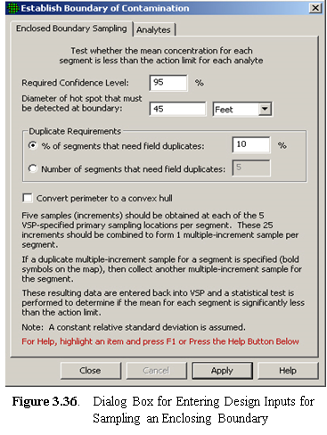
Menu selection Sampling Goals > Establish Boundary of Contamination > Enclosing Boundary brings up the dialog box in Figure 3.36 for tab Enclosed Boundary Sampling The first input required is the confidence needed that the mean calculated from limited sample data is indeed less than the action limit. For this example, that confidence level is 95%.  The diameter of the area of contamination (i.e., the hot spot) that the user wants to be sure is detected at the boundary is input as 45 ft. The next box, labeled Duplicate Requirements, has to do with how many of the segments need duplicate MI samples to be collected. VSP requires that: at least 5 segments; or at least 10% of the segments, need duplicates. The user may select which requirement is used. While 10% is the minimum, the user may input any percentage for duplicates.

Note: The purpose of duplicate MI samples is to estimate the relative standard deviation of the data so that an Upper Confidence Limit (UCL) test can be conducted for each segment. See VSP Help for more information.

If the boundary of the site is very irregular, e.g., has various indentations, the VSP user can specify in the dialogue box that VSP should change the boundary to a convex hull. This has the effect of smoothing out the boundary irregularities, but it also enlarges the area enclosed by the initial boundary. In practice, the VSP user can try this option and view the resulting initial boundary to see if the new boundary is acceptable. In Figure 3.36 we leave this box unchecked.

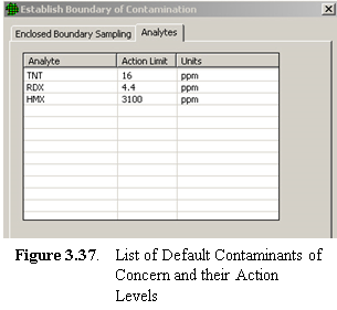The user now must input the contaminants of concern and the threshold (action level) at which we want VSP to trigger extending the contamination boundary line. The dialog box for tab Analytes is shown in Figure 3.37. VSP provides a default list of contaminants of concern (TNT, RDX, and HMX) and a default list of upper limit values (Action Limit) for each (16ppm, 4.4ppm, and 3100ppm). To remove a contaminant from the list, erase the name and the limit. To add a contaminant, enter its name and threshold value in the blank lint below the last contaminant.

For the Millsite.dxf map file selected, and the central ellipse in the center of the map selected as the Sample Area with an enclosing boundary, we see in Figure 3.38 that after clicking the Apply button in the previous screen, VSP divides the boundary into 12 segments. Shown are the 5 equally-spaced Primary Sampling Locations in each of the segments. The segments for which the Primary Sample Locations are in bold type will have duplicate samples taken at each location. Different symbols are assigned to each segment to differentiate the segments visually.  For each segment, VSP assumes the user will 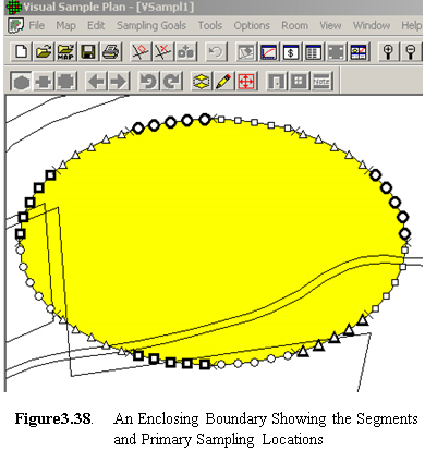form the MI sample for that segment by mixing 5 small soil samples collected from each of the 5 Primary Sampling Locations. Hence, each MI sample is formed from the 25 small soil samples.

The user now collects the samples, mixes the samples to form a representative MI sample for each segment, and measures each MI sample. The results are input into VSP using the Sample Information box that appears when the cursor is placed over one of the Primary Sample Locations, and right-click the mouse. Use the keyboard to enter the measurement value into the appropriate row in the column labeled "Value" in the Segment Sample Results sub-box. Use the down arrow button on the keyboard to move between rows within the sub-box.  Figure 3.39 shows the Sample Information Box.

We happened to click on a segment for which two MI samples are required. Thus, we will need to input two sets of measurements, one for each of the 3 analytes, making 6 input values required. Click the OK button on the dialog box to close the Sample Information box for that segment. Repeat the above process for each of the segments to enter all the measurement values.  The Segment Sample Results box has a column headed "UCL". VSP will fill in this box with the Upper Confidence Limit on the mean once all the measurement values for the segment are input. The UCL is used to test whether the mean exceeds the action level for that segment.

Sample results can be entered into VSP using software such as a spreadsheet. Consult VSP's Help for instructions on this process.

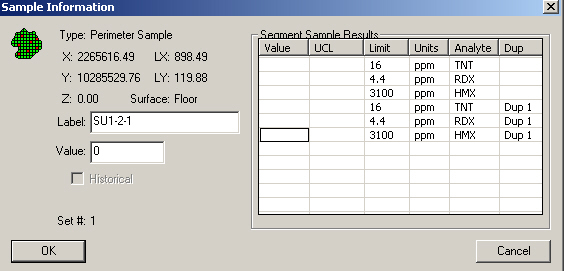
Figure 3.39.   Sample Information Box for Entering Data into VSP, Duplicate Samples Required

VSP now tests whether each boundary segment should be enlarged (bumped out). This is described in an Appendix to the report PNWD-3580 referenced above. In Figure 3.40 we see an example of two expanded boundaries. Note the red colored Primary Location Segments indicate that segment did not pass the UCL test and hence had to be "bumped out".

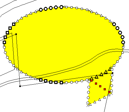
Figure 3.40.   Enclosed Boundary with Two Bumped-Out Segments

3.2.12.2 Partial Boundaries

The input screens, the dialog boxes, and the maps for Partial Boundaries problems are similar to those for the Enclosed Boundaries and will not be shown here. For a discussion of the Partial Boundaries problem consult the VSP Help function.

For detailed documentation on establishing boundaries of contamination, please refer to the VSP Help Topic Establish Boundary of Contamination.

3.2.13 Sampling Within Buildings

While many of the sampling designs presented in earlier sections could be applied to 3-dimensional sample areas such as building and rooms (-- as opposed to 2-dimensional sample areas such as land areas), the sampling designs provided under Sampling within a Building are uniquely suited for problems where contamination is released into an enclosed structure and contamination can be on walls and ceilings, windows and doors, as well as on floors, on and under furniture, etc.. Many of the VSP features added for this module were requested by the Department of Homeland Security (DHS), Combating Terrorism Technology Support Office. DHS wanted ways to sample walls, floors, ceilings, and other surfaces to determine if contamination is present, its magnitude and extent throughout the building, and ways to sample after decontamination to see if the decon was effective.

The sub-goals within this section work through various scenarios when a chemical, biological or radionuclide release has occurred within a building. Contamination may be isolated, microscopic, and may selectively adhere to surfaces and crevices. It may be capable of being spread throughout the building, may pose a health risk at very low levels of contamination, and may be from an unknown source and released in an unknown location within the building. The unique nature of these contamination scenarios requires unique sampling methods and unique analysis methods. In the case of a terrorist bio/chem/rad event, the parameters of interest will most likely be the mean, maximum, or a percentile of the distribution of all possible measurements. Depending on what the goals are, different sampling designs will be suggested. 

3.2.13.1 Compare Average to a Threshold

A threat analysis team would be interested in average contamination within a building or room if the primary exposure scenario concerned an accumulated dose, or a long-term exposure of individuals randomly moving about within the room/building. The sampling goal would be to take samples and compare the average contamination in a room, or a group of rooms, to a health risk-based threshold. 

A number of statistical sampling designs could be applicable depending on the assumptions, constraints, and sampling technologies. These designs include simple random sampling, grid sampling, sequential sampling, and collaborative sampling. Similarly, a number of tests could be conducted on the data to decide if the mean is greater than a threshold. These tests include the one-sample t test and the sign test. The designs for the sampling goal of comparing an average to a threshold have been discussed earlier in the manual under the sampling goal of Compare Average to Fixed Threshold (Section 3.2.1).

3.2.13.2 Show That At Least Some High % of the Sampling Area is Acceptable

Most biological, chemical, or radiological threats involve a risk to an individual if any exposure to the contaminant is encountered. Other threats may depend on how much of a room or set of rooms is contaminated above some action level (AL). As such, there is an interest in individual (rather than average) measurements. If the entire area/decision unit cannot be surveyed, the goal may be to take limited samples and based on those samples, make statements (with the associated confidence level) about unsampled areas. Another goal might be to make a confidence statement about the percent of the total population that is contaminated, based on sample data. For each goal, one of the VSP outputs is a statement that can be made based on sample results. For example, for the sampling goal Sampling within a Building > Show that at least some high % of the sampling area is acceptable > Using presence / absence measurements, there are several methods which provide X%/Y% confidence statements, where we are X% confident that no more than Y% of the sampled area is unacceptable provided the number of sampled grid cells which can be unacceptable has not been exceeded.

3.2.13.2.1  Using Presence/Absence Measurements

Case 10. In VSP, open the VSP project file "apartment.vsp" by selecting File > Open Project and selecting the file. Three rooms are selected in the project file. We are tasked with sampling these rooms to check for a contaminant. The contaminant is dangerous if humans have any exposure to it, so none of the grid cells in the rooms can be unacceptable. We have no prior information about the release to establish prior beliefs or to determine if any grid cells are more likely to be contaminated than others. Initially the desire is to be 99% confident that 100% of the area is not contaminated. To view the walls and ceilings of all three rooms, you can select View > 3D and zoom in to view all surfaces. 

VSP Solution 10: We start by choosing the VSP Sampling Goal option of Sampling within a Building > Show that at least some high % of the sampling area is acceptable > Using presence / absence measurements. Enter the Parameters as shown in Figure 3.41.

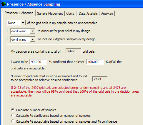
Figure 3.41. Parameter Inputs for Case 10

We see that for our inputs, nearly all of the grid cells in the apartment must be sampled, 2473 out of 2497. This is largely because we require that 100% of the grid cells be acceptable. If we change this to "at least 99%" of all the grid cells are acceptable", 419 grid cells must be sampled and be acceptable for us to state we are 99% confident that at least 99% of the area is acceptable. This demonstrates the power of sampling using X%/Y% confidence statements. To achieve 100% confidence or state that 100% of an area is acceptable, most of the grid cells will need to be sampled. However, when these parameters can be adjusted slightly below 100%, the number of samples can be greatly reduced.

Case 11.  Now assume that sample collectors know from previous experience that when the entire area is not saturated with contaminant, grid cells in certain portions of the apartment are more likely to be contaminated than other grid cells. Sample collectors want to take 40 judgment samples which are 3 times as likely to be contaminated than other grid cells. How many additional random samples must be taken for us to be 99% confident that at least 99% of the grid cells are acceptable?

VSP Solution 11:  Select that we "want" to include judgment samples in our design and enter the parameters as shown in Figure 3.42. The knowledge that our 30 judgment samples are 3 times as likely to be contaminated reduced the total sample size from 419 to 350, a difference of 69 samples.

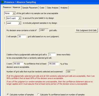
Figure 3.42. Parameter Inputs for Case 11

Case 12:  Now assume that sample collectors have previously sampled areas outside and adjacent to the apartment, and these areas have been cleared. Using their professional experience and judgment, they are already 90% confident that none of the apartment will be contaminated. They will again take 30 judgment samples which are 3 times as likely to be contaminated as other grid cells. How many samples must now be taken to be 99% confident that at least 99% of the area is acceptable?  What happens if we reduce the confidence statement to being 95% confident that at least 99% of the area is acceptable? What about 95% confident that 95% of the area is acceptable.

VSP Solution 12:  Select that we "want" to account for prior belief in our design and enter the parameters as shown in Figure 3.43. We see that the number of samples has been reduced from 350 to 330 using the prior information that sample collectors were already 90% confident that most of the area would be acceptable. 

Changing the confidence level to 95% further reduces the total number of samples from 330 to 192. The desired confidence is a key driver in compliance sampling.

Changing the X%/Y% confidence statement to being 95% confident that at least 95% of the area is acceptable yields a value of "NA" for the number of random samples to be collected. This implies that the 30 judgment samples being collected satisfies the sampling requirements for the current sampling design. This is only valid if the statements we make about prior beliefs and judgment sampling locations are correct. These examples have demonstrated that prior information can drive down sample sizes. Like all sampling designs, it is important to be sure that assumptions are accurate. Prior beliefs should only be adjusted if there is evidence and experience that supports it, and not be changed solely for reducing sample sizes. 

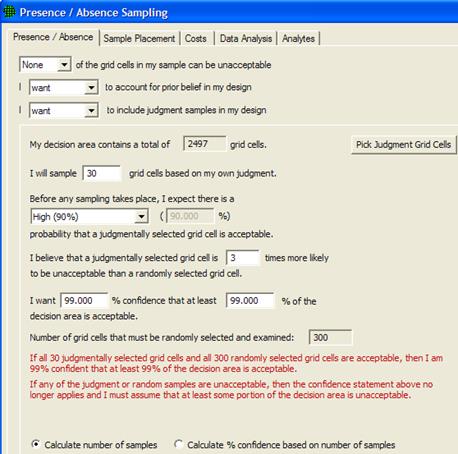
Figure 3.43. Parameter Inputs for Case 12

All of the presence/absence examples presented thus far have been designed so that if any of the samples are unacceptable, we conclude the area is unacceptable. There is another option where one or more samples are allowed to be unacceptable. This may be useful in situations where the contaminant of interest is known to not be dangerous when it is only sparsely located. For this case, we would select "Some" of the grid cells in my sample can be unacceptable. In addition to the X%/Y% parameters in other sampling designs, you also enter the Beta level and associated percentage of the site that is contaminated if we were to assume the alternative hypothesis is true that the area is acceptable. This design calculates the total number of samples you would need to take to make these confidence statements if the number of unacceptable samples was the number specified. If the number of grid units in the sample that are unacceptable exceeds the Acceptance Number, C (which VSP calculates), then the user concludes the maximum acceptable % of grids contamination has been exceeded and the real proportion defective is equal to or greater than Pa. The method used for this design is called "Acceptance Sampling for C > 0", or just "Acceptance Sampling". Acceptance Sampling is a test of hypothesis between two different statements about the number of defective units in the population, Do and Da (Da > Do). Therefore, Acceptance Sampling for C > 0, requires both an Alpha and a Beta (see Section 3.2). Refer to the Help for a more complete discussion of the method.

A scenario when Acceptance Sampling for C > 0 may be applicable is that you know some level of contamination may exist (naturally occurring, or the level of contamination is at the detection level of the monitoring equipment) to give a lower bound Po, the probability of a defective unit given Do defective units are in the population. There is an upper bound Pa (probability when there are Da defective units) where a health risk may occur and you want to be have a high confidence of detecting contaminating greater than Pa percent. 

3.2.13.2.2  Using Quantitative Measurements that Follow a Normal Distribution

If the decision unit is large, and the sample support (the amount of material contained in the sample, or the area swiped for a sample) is small, then point samples are taken under the assumption of an infinite population of possible sample locations. The assumption of an infinite population eliminates the need for a finite population correction factor in the sample size calculation. It also eliminates the need to consider sampling with or without replacement. Random points are generated in the decision unit and samples are taken at those points.

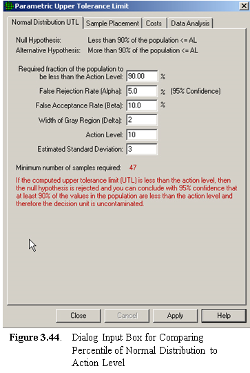Methods associated with infinite populations are concerned with percentiles of a population. To test the null hypothesis that the decision unit is contaminated, we say that if the upper confidence limit on a percentile of the population is less than the limit, then we can reject the null hypothesis and conclude the decision unit is uncontaminated. A confidence interval on a percentile of a population is called a tolerance interval. The tests in this group calculate an Upper tolerance limit (UTL) for the population and compare it to a limit. The UTL is calculated from sample results. The methods of Upper tolerance limit are used for infinite populations.

If the decision unit (i.e., a room) is small relative to the sample support, and the sample support is well-defined (say the sample will consist of a 4 inch square swab), then samples are taken under the assumption of a finite population of all possible sample locations. We would partition the room into individual, non-over-lapping "grid" locations, specify the total number of grids in the room, specify the number of grids to be sampled, then use a random selection of size n (calculated by VSP) grids to be included in the sample.

Methods associated with finite populations use the concept of "lots", i.e., a discrete group of units extracted from a total production run. This has application to a decision unit that can be gridded, with each grid unit having a discrete identity within the larger population. The methods of Acceptance sampling (taken from industrial quality control) are used for finite populations. The tests in this group of methods count the number of grids in the sample that exceed an action level (are defective) and as long as that number is less than or equal to an "Acceptance Number", we say the level of contamination is within the tolerable (i.e., acceptable) limits.

If the distribution of measurements of contamination at all possible point sample locations in the decision unit can be considered to be normally distributed (i.e., the standard bell-shaped curve), we can use the formula that calculates the UTL of a percentile of the normal distribution in the test of the null hypothesis. This UTL will be compared to the Action Level to determine whether we accept or reject the null hypothesis. The UTL formula will also be used in the calculation of the sample size, n. Figure 3.44 shows the dialog box for this sampling goal. The design using a parametric upper tolerance limit is select from Sampling Goals > Sampling within a Building > Show that at least some high % of the sampling area is acceptable > Using Quantitative Measurements that Follow a Normal Distribution.

The null hypothesis being tested is that the true P^th percentile of the population exceeds a fixed Action Level (i.e., the decision unit is contaminated). The user is asked to input the smallest fraction of the population required to be less than the Action Level in order for the unit to be considered uncontaminated, input here as 90%. Note: none of the designs discussed below use the Action Level in the sample size calculation, but Action Level is used in performing the Tests under the Data Analysis tab (see Section 5.6 on Data Analysis). The next set of inputs is the DQO inputs required to calculate sample size. These inputs are defined in Section 3.2.  The Help brings up a screen that describes how these inputs are used to calculate n. VSP calculates that 47 samples are required to execute the test of the hypothesis with the set of DQOs listed.

In Figure 3.45 we see the 47 samples located in a room. We drew a room, supplied the inputs for the Dialog Box, and hit the Apply button. We select View > Room to see the samples located in the room.

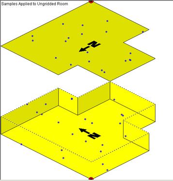
Figure 3.45.   Samples Placed on Floor and Ceiling Within a Room

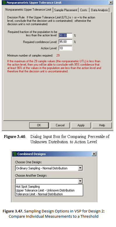3.2.13.2.2  Using Quantitative Measurements From an Unknown Distribution

If the distribution of measurements is unknown, we must calculate a non-parametric UTL for use in the test of the hypothesis that the true Pth percentile of the population exceeds a fixed Action Level. This is accessed from Sampling Goals > Sampling within a Building > Show that at least some high % of the sampling area is acceptable > Using Quantitative Measurements From an Unknown Distribution. The non-parametric UTL happens to be the largest measurement of the n samples taken, where n is calculated using the DQO inputs in Figure 3.46 and the sample size formula discussed in the VSP Help for this input screen.

VSP calculates that we need to take 29 samples in order to make a 95% confidence statement about the 90th percentile of non-parametric distribution. The exact wording of the conclusion that can be drawn is one of the outputs of VSP. An example conclusion is shown in red in Figure 3.46.

3.2.13.3 Detect Hot Spots

The 3-dimension scenario for the hotspot problem is that the user is concerned about hotspots on ceilings as well as on floors and walls. The extension from the 2-dimensional problem is straightforward. The floor, ceiling and wall-strip (wall sections laid edge-to-edge) represent three independent surfaces that might contain a hotspot. Refer to Section 3.2.8 Locating a Hot Spot for a discussion of this sampling goal.

3.2.13.4 Combined Average and Individual Measurement Criteria

In many of the scenarios associated with contamination within a building, the user may be concerned about average contamination greater than a threshold for purposes of assessing chronic exposure of individuals to contamination over an extended period of time and over broad areas, yet also want to be assured that no individual measurement exceeds a different threshold. Or the user may want to be assured no hotspots of a certain diameter exist, and that no individual measurements exceed a threshold. The user wants to take enough samples to meet both goals, so the sample size taken will be the larger of that required by either design. The larger-than-required sample size for the smaller design will result in improved performance, such as

• a smaller Beta error rate, applicable for most of the testing designs (e.g., One Sample T, WSR),

• a higher-than-requested confidence for the Nonparametric UTL design, and

• a smaller size for a detectable hot spot for the Hot Spot design.

VSP back-calculates these performance variables for the larger sample size and displays the new values for the performance variables in the Dialog Box(s). This is accessed by selecting Sampling Goals > Sampling within a Building > Combined average and individual measurement criteria.

Figure 3.47 shows the Dialog Box for choosing the two designs for the Combined Design Goal. The two designs selected will appear in separated windows adjacent to the "Combined Designs" window.

The Hot Spot design is included in the options for both Design 1 and Design 2 to allow the user to choose the combined goals of detecting Hot Spots and Compare Individual Measurements to Threshold. For the Combined Designs Dialog to work properly, the Dialog Boxes for Design 1 and Design 2 must be open. You have to close the Combined Designs Dialog before you can close either of the two individual Design Dialogs.

For detailed documentation on building sampling, please refer to the VSP Help Topic Building Sampling.

3.2.14 Radiological Transect Surveying

Radiological transect surveying is supported in VSP. Most of the methods leverage methods originally implemented in VSP for transect sampling for the detection of unexploded ordnance. For this reason, we will not go into great depth here as these methods are explained later in Chapter 7. 

3.2.14.1   Transect Spacing Needed to Locate a Hot Spot

These methods refer to cases where nearly-continuous measurements are taken along transects (lines or swaths) and tightly-spaced readings are automatically logged or stored electronically. Because of this tight spacing, the sampling design for whether or not a transect traverses a hot spot is very robust for the similar problem of whether or not a radiological survey measurement is taken within a hot spot. The sampling designs for "Ensure high probability of traversal" and "Manual transect spacing" from the UXO modules are utilized here. For more information, see VSP's Help topic under Sampling Goals > Radiological Transect Surveying > Transect spacing needed to locate a hot spot.  Chapter 7, the UXO methods chapter, also explains how to use these methods, albeit with slightly different terminology. 

3.2.14.2 Locate and Mark Hot Spots

This analytical method simply marks points on the map where measurements taken exceeded a specified threshold.

3.2.14.3 Geostatistical Analysis

Geostatistical analysis of radiological survey data is similar to that of methods for analyzing well locations on a map. The exception is that radiological surveys can contain many, tightly spaced point samples. For more information on Geostatistical Analysis, see the Help section in VSP for this module. Chapter 7 also contains some material on Geostatistical Analysis.

3.2.14.4 Post-Survey Probability of Sampling Within a Hot Spot

This module uses simulation to compute the probability that a survey would have sampled inside a hot spot of a given size and shape (but unknown location). The user specifies a hot spot of a certain shape and size on the "Hot Spot" tab as in VSP's UXO modules. On the "Hot Spot Traversal Simulation" tab, the user specifies the number of simulations to run. VSP places the center of a hot spot randomly that number of times within the sample area, and for ellipses generates a random angle of orientation. The hot spot is traversed if one or more survey measurements lay within the hot spot. The percent of hot spots detected is reported as a percentage.

For detailed documentation on radiological transect surveying, please refer to the VSP Help Topic Radiological Transect Surveying.

3.2.15 Item Sampling

This module uses the same statistical model as the Compliance Sampling for Presence/Absence module explained earlier in this chapter. The only difference is that this module uses terminology and visualizations adapted to sampling of discrete items rather than sampling grid cells on surfaces.

3.2.16 Detecting a Trend

The purpose of the Mann-Kendall (MK) test (Mann 1945, Kendall 1975, Gilbert 1987) is to statistically assess if there is a monotonic upward or downward trend of the variable of interest over time. A monotonic upward (downward) trend means that the variable consistently increases (decreases) through time, but the trend may or may not be linear. The MK test can be used in place of a parametric linear regression analysis, which can be used to test if the slope of the estimated linear regression line is different from zero.  The regression analysis requires that the residuals from the fitted regression line be normally distributed; an assumption not required by the MK test, that is, the MK test is a non-parametric (distribution-free) test.

Hirsch, Slack and Smith (1982, page 107) indicate that the MK test is best viewed as an exploratory analysis and is most appropriately used to identify stations where changes are significant or of large magnitude and to quantify these findings.

To calculate the sample size required for performing a Mann-Kendall test, the dialogue is accessed from Sampling Goals > Detect a Trend > Residuals not required to be normally distributed > No Seasonality. A sample dialogue is shown in Figure 3.48. 

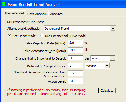
Figure 3.48.  Mann Kendall Design Dialog

We have the options of specifying if we want to detect an upward or downward trend, or both. A linear model is used if the change over time is expected to be steady. If the change over time is expected to follow more of a curvilinear pattern, an exponential curve may be a better choice.  In Figure 3.47 we want to detect a downward trend of -1 units per year. VSP calculates that given our input parameters, we would have to sample for 34 sampling periods (34 months in this case) to collect enough data for conducting a Mann-Kendall test. 

If you suspect there may be seasonal fluctuations in the data, select Sampling Goals > Detect a Trend > Residuals not required to be normally distributed > Seasonality. In the Seasonal-Kendall test, it is assumed that sampling is conducted every season. Other than defining the seasons, the dialogue is very similar to the dialogue for the Mann Kendall test with no seasonality.

Figure 3.49 shows a data analysis window for the Seasonal-Kendall test. The "Testing for Global Trends" alerts you if trends differ by season or if there are differences between sampling locations. If either is the case, then the Seasonal Kendall test results could be misleading. In this case, there appear to be no global trends, so the downward monotonic trend detected appears to be valid. 

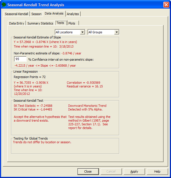
Figure 3.49. Data Analysis for Seasonal Kendall Test

Trend Data is often easiest to use by looking at a Time vs. Data plot (Figure 3.50). The raw Values or model Residuals are plotted against the time variable to help visualize trends over time. In VSP, there are several options available for customizing the plot:

Show CI: Checking this box allows the user to enter a confidence level. Assuming the model fit is good, a confidence interval and prediction interval are displayed around the fitted line. The confidence interval (CI) illustrates the estimated variability around the fitted line. The prediction interval (PI) is a wider interval which identifies a range in which the number of raw values that fall in the interval is approximately the percent specified for the confidence level. 

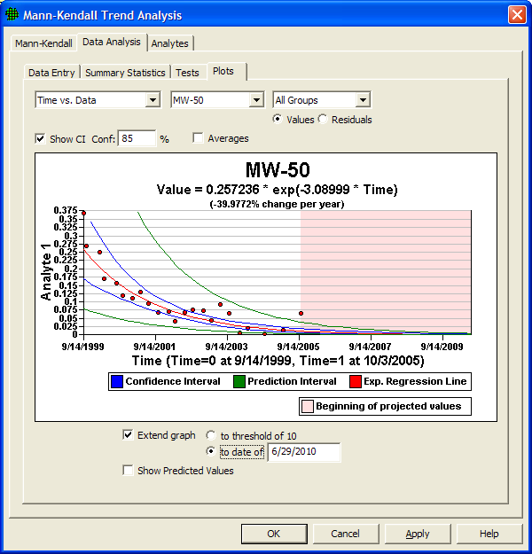
Figure 3.50.  Time Vs. Data Plot in VSP

Averages: Checking this box allows the user to enter a time interval for which to average points. VSP displays the averages for the time intervals instead of showing all of the raw values. This can be a useful way to view data when there is a large amount of data on the plot.

Extend Graph: This allows the user to extend the graph to visualize where the model would extend if we were to extrapolate that future events will follow the trend.

Show Predicted Values: This allows the user to display a column of predicted values generated by a model outside of VSP. This is done by importing the column and specifying it as a "Predicted" column while importing. 

For detailed documentation on detecting a trend, please refer to the VSP Help Topic Detect a Trend.

3.2.17 Identify Sampling Redundancy

The well redundancy modules in VSP are used for identifying redundant wells, and for identifying a technically defensible temporal spacing of observations for wells. 

3.2.17.1 Analyze Spatial Redundancy

The spatial redundancy module in VSP is based on a geostatistical analysis of well locations. The algorithm is based on the accumulation of kriging weights to determine a global kriging weight associated with each well. The global kriging weight for a given data point is determined by adding the kriging weights for that data point for all locations in the kriging grid. Global kriging weights had previously been used by Isaaks and Srivastava (1989) as a method of providing global weights for individual data points. Cameron and Hunter (2002) used global kriging weights to identify the relative importance of wells in mapping contaminant plumes, and to identify wells that could be removed from the sampling schedule. 

In VSP, wells are ranked in terms of their contribution to the plume map through the global kriging weight, and the lowest ranked data location is removed from the data set. The kriging and ranking process is then repeated until the maximum number of wells is removed from the data set. At each iterative step, the program calculates the root mean square error (RMSE) between the base plume map and the plume map generated after a given number of wells have been removed. The user then evaluates the number of wells that can reasonably be removed from the sampling schedule by examining the plot of RMSE versus the number of wells removed. In addition, maps showing the plume maps generated using the base case (all wells) can be compared with plume maps generated after eliminating a given number of wells.

The analysis is performed using a normal score transform of the data. Transformation of contamination data is often needed because of their tendency to be highly skewed (Gilbert 1987). The normal score is widely used in geostatistics because of its ability to transform data with any distribution into a variable with a perfectly normal (i.e., Gaussian) distribution (Deutsch and Journel 1998). The normal score transform is also used in the Probability and Uncertainty Mapping module in VSP.

The well redundancy module includes several steps:

1.   Examine data using data analysis tools and maps

2.   Calculate variogram

3.   Fit variogram model

4.   Determine kriging parameters

5.   Complete the well analysis

a.    Go to Analyze Wells tab

b.    Choose maximum number of wells to eliminate from sampling schedule

c.    Hit start to begin process

d.    Review results

e.    Select number of wells to eliminate from sampling schedule

Steps for Analysis of Redundant Wells using VSP

Step 1 - Examine the data

Before beginning, the data should be examined to ensure that geostatistical analysis is appropriate. At least 30-50 data points are recommended, and some authors have suggested that the minimum number of data needed is as much as 100 (e.g., Webster and Oliver 1993), especially for data that exhibit a large amount of short range variability.

Use the Data Analysis module under the Tools menu in VSP to check for extreme outliers and see whether the data follow a highly skewed distribution. Kriging also requires the assumption that the data are spatially continuous, which will be determined during the variogram analysis. 

The Exclude column on the Data Entry tab is a binary indicator that indicates whether or not a data point should be included in the variogram calculations. The user might set the Exclusion indicator to 1 (i.e., exclude the point) if a data point is highly redundant. An example might be the large number of wells present along a remediation barrier.  It might be useful to exclude such a large number of highly redundant points because they can dominate the variogram. The user can calculate the variogram both with and without points marked for exclusion.

The Reserved column on the Data Entry tab is a binary indicator for whether or not a well should be included in the well redundancy analysis. In some cases there may be wells that cannot be dropped from the sampling schedule, for regulatory or other reasons. In that case, they can be included as data points in kriging, but would not be included in the list of wells that could be removed from the sampling schedule, even if they appear to be redundant.

Step 2 - Calculate the experimental variogram

What is a variogram? A variogram is a description of the spatial continuity of the data. The experimental variogram is a discrete function calculated using a measure of variability between pairs of points at various distances. The exact measure used depends on the variogram type selected (Deutsch & Journel 44-47).

The distances between pairs at which the variogram is calculated are called lags. For instance, lags may be calculated for samples that are 10 feet apart, then samples that are 20 feet apart, then 30 feet, etc. In this case the distance between lags is 10 feet. Since points may not be spaced exactly 10 or 20 feet apart, the lag settings include a lag tolerance value that is typically set to half of the distance between lags. For the previous example, that would mean that the first lag would include all pairs of points that are between 5 and 15 feet from each other.

Variogram Parameters

Variogram type: 

Select the type of empirical variogram to calculate. The default and recommended first choice is Semivariogram. Other types can be better for skewed distributions or with the presence of extreme values. For example, the Semivariogram of logarithms uses logarithmic transform of the data, and therefore can be useful for log-normally distributed data. The Semivariogram of normal scores uses a normal score transform of the data (Deutsch and Journel 1998), which can also be helpful for highly skewed data.

Lag Settings: 

Number of lags: Specifies how many lags of the variogram to calculate. This, together with the distance between lags, determines the maximum distance between pairs of points at which the variogram is calculated. This maximum distance is called the variogram coverage (number of lags times the distance between lags), and is displayed on the dialog. The variogram coverage should be less than the site size, and a good guideline is for the variogram coverage to be closer to ½- ¾ of the site size.

Distance between lags: The intervals to calculate lags. A good distance between lags should be no smaller than the shortest distance between data points, and should be close to the average spacing of samples. The ideal lag spacing includes roughly the same number of pairs in each lag, and at least 30 pairs for each lag.

Lag tolerance: How much the distance between pairs can differ from the exact lag distance and still be included in the lag calculations. The default is ½ of the distance between lags, which ensures that all possible pairs are included.

Step 3 - Fit a variogram model

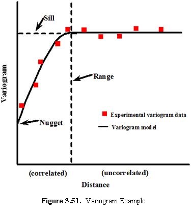Because the kriging algorithm requires a positive definite model of spatial variability, the experimental variogram cannot be used directly. Instead, a model must be fitted to the data to approximately describe the spatial continuity of the data. Certain models (i.e., mathematical functions) that are known to be positive definite are used in the modeling step.

Figure 3.51 shows an experimental variogram with a variogram model fitted to it. Each red square is a lag of the experimental variogram. The x-axis represents the distance between pairs of points, and the y-axis represents the calculated value of the variogram, where a greater value indicates less correlation between pairs of points. This particular variogram shows a spatial relationship well suited for geostatistical analysis since pairs of points are more correlated the closer they are together and become less correlated the greater the distance between points. 

Figure 3.51 also illustrates three important parameters that control the fit of the variogram model. The nugget is the y-intercept of the variogram. In practical terms, the nugget represents the small-scale variability of the data. A portion of that short range variability can be the result of measurement error. 

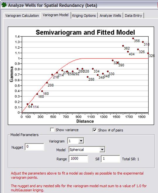
Figure 3.52.  Semivariogram and Fitted Model and VSP

The range is the distance after which the variogram levels off. The physical meaning of the range is that pairs of points that are this distance or greater apart are not spatially correlated. The sill is the total variance contribution, or the maximum variability between pairs of points.

VSP can display the number of pairs that went into calculating each variogram lag. There should be at least 30 pairs for each variogram point, if there are fewer this could indicate that the distance between lags should be increased, so that more pairs are included in each lag. 

The model type, nugget, sill and range can all be modified to fit the variogram model. Primary importance should be given to matching the slope for the first several reliable lags. An example from VSP is shown in Figure 3.52.

Nugget:  Related to the amount of short range variability in the data. Choose a value for the best fit with the first few empirical variogram points. A nugget that's large relative to the sill is problematic and could indicate too much noise and not enough spatial correlation.

Model type: See Deutsch & Journel for the details of these models. Spherical and exponential are most widely used.

Range: The distance after which data are no longer correlated. About the distance where the variogram levels off to the sill.

Sill: The sill is the total variance where the empirical variogram appears to level off, and is the sum of the nugget plus the sills of each nested structure. Variogram points above the sill indicate negative spatial correlation, while points below the sill indicate positive correlation. The variance of data can be used as a reasonable default. The variogram may not exhibit a sill if trends are present in the data. In that case, geostatistical analysis should proceed with caution, and at the least, ordinary kriging should be used for mapping.

Variogram number: By default a single variogram model is used, but up to three can be nested to more accurately fit a model to the data. In cases where nested scales of spatial continuity appear to be present, it is best to attempt to determine the scientific reason for the multiple nested models (e.g., a short range might be related to the average dimensions of point bars, with a longer range related to the dimensions of a flood plain in which the point bars are distributed).

Step 4 - Determine the kriging parameters

The kriging algorithm estimates concentration over a regular grid across the site, and the sum of the kriging weights are used to determine the overall weight assigned to each data point. For a particular grid location, the surrounding data points within a specified search window are used to calculate the estimated concentration. The kriging parameters define that grid and search window, and determine how the kriged estimates are calculated. The different kriging options in VSP are shown in Figure 3.53.

Grid size: Determines the resolution of the concentration estimate map. The ideal choice depends on the application and the data distribution, but it is important to ensure that the grid size is not too small relative to site size, since that would require a large number of estimates to be calculated and could result in a long execution time.

Kriging type: Ordinary kriging re-estimates the mean within the local search area, this can help account for trends in the data. Simple kriging uses a constant, site-wide mean, so should only be used if the data distribution and variogram support that assumption. 

Number of points to use: Minimum and maximum number of data points within the search window to be used in kriging each estimate. If there isn't at least the minimum number of points within the search ellipse, no estimate will be calculated. The maximum number of points to use can also be specified to limit the computational time required.  Larger maximum numbers increase the size of the matrices that are inverted for the estimation of each grid node, which increases the computational time.

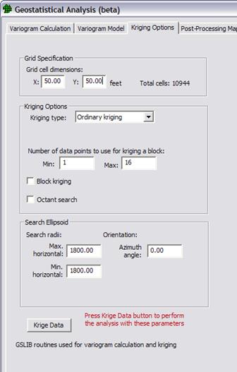Block kriging: Estimates concentrations for blocks of a specified size instead of a grid of points. Point kriging is more commonly used in environmental applications.

Octant search: If octant search is enabled, the search ellipse is divided into eight equal-angle sectors, and only the specified maximum number of points from each octant will be used. 

Search ellipsoid: These parameters determine how far out to search for data to support a particular kriged estimate.

Max and min horizontal radii:  These are the semi-major and semi-minor axes of the search ellipse, respectively.  They each should be greater than the range of the variogram model.  These values should only need to differ (i.e. define an ellipse instead of a circle) if anisotropy is present. Changing the azimuth angle defining the orientation of the search ellipsoid is also only necessary for a site with anisotropy. 

Step 5 - Complete the well analysis

The analyze tab allows a choice of the maximum number of wells to remove in the analysis. The default is all wells available for analysis. If the maximum to be removed is less than the total number of wells, which will almost always be the case, the total execution time will be reduced.

After choosing the maximum number of wells to be removed, start the analysis. If the execution appears to be extremely slow, e.g., a minute passes between each iteration that removes a well, hit the Stop button, and return to the Kriging tab to increase the size of the X and Y grid cell dimensions.

Once the iterative process is complete, and the wells have been ranked in order of their value, select "View Maps" (bottom of Figure 3.54) to examine the base map and the map generated with a selected number of wells removed. There is no objective measure to determine how many wells can be removed. However, examination of the RMSE plot provides a measure of the increase in RMSE for removal of each well, and may suggest thresholds at which large increases in RMSE occur for selection of additional wells. That, coupled with comparison of maps for different numbers of removed wells, can be used to select the best number of wells to remove that will decrease sampling costs without adversely impacting the ability of maps based on the remaining data to adequately represent the plume. 

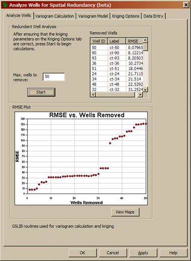
Figure 3.54. Redundant Well Analysis

3.2.17.2 Analyze Temporal Redundancy

The temporal redundancy module in VSP provides methods for examination of the temporal spacing of observations. The object of the module is to identify a technically defensible temporal spacing. There are two different sampling goals that are addressed here. One of the main goals is determining if fewer observations could be used to characterize the contaminant concentrations at a well over time. A second objective that is sometimes needed is to identify the minimum temporal spacing between observations so that they are independent from one another. Methods are included in the module to address both objectives. 

Before performing the analysis, the user may wish to clean the data. The Data Preparation tab in the Temporal Redundancy module includes tools to select wells for inclusion in the analysis and to remove large temporal gaps and outliers that may be present in the data.

Single well analysis - Iterative thinning 

The iterative thinning approach is based on an algorithm published by Cameron (2004). The goal of the algorithm is simple, yet elegant: identify the frequency of sampling required to reproduce the temporal trend of the full data set. The trend may include simple upward or downward trends, but the algorithm also allows reproduction of more complex patterns, e.g., cyclical patterns related to seasonal variations in concentration. 

The median temporal sample spacing between historical observations is first calculated and used as the baseline sample spacing. The iterative thinning algorithm uses the Lowess algorithm to fit a smooth trend and confidence bands (Cleveland 1979) around the full temporal data set. A default bandwidth of 0.5 is used. See LOWESS Plots for information on the equations used to fit the smooth trend and calculate the confidence bands around that trend. A percentage of the data points are removed from the data set and Lowess is used with the same bandwidth to fit a smooth trend to the reduced data set. 

The ability of the reduced data set to reproduce the temporal trends in the full data set is evaluated by calculating the percentage of the data points on the trend for the reduced data set that fall within the 90% confidence interval established using the full data set. Increasing numbers of data points are removed from the data set and each of the reduced data sets is evaluated for their ability to reproduce the trend observed in the full data set. A default level of 75% of the points on the trend for the reduced data falling within the confidence limits around the original trend is deemed acceptable (Cameron 2004). In order to guard against artifacts that might arise from the selection of a single set of data points to remove, the iterative removal process is repeated a large number of times (default number of iterations is 500). The proportion of data that can be removed while still reproducing the temporal trend of the full data set is used to estimate an optimal sampling frequency.

Single well analysis - Variogram analysis

The use of variogram analysis for analysis of temporal redundancy has been discussed by several authors, including Tuckfield (1994), Cameron and Hunter (2002), and Cameron (2004). The first step is to calculate a temporal variogram for well concentrations, and then fit a variogram model to the experimental variogram. Given the definition of the range of the variogram model as the lag distance beyond which data are no longer correlated, the variogram range was proposed by Tuckfield (1994) as an estimate of a technically defensible sampling frequency. 

It should be noted that the goal of that approach was to provide sets of independent samples that could be used for credible comparisons (e.g., hypothesis testing) of up gradient and down gradient wells (Tuckfield 1994).  This would require sampling that would be no more frequent than the temporal variogram range, so that independent samples would be obtained. This is a valid sampling design goal and for that reason, the use of variogram analysis is a valid approach for identifying a defensible temporal sampling frequency. However, it should be noted that the use of the temporal variogram approach would not define a sampling frequency that would be best for identifying any temporal trends in the data. If that is the goal of the analysis, then the iterative thinning approach described above would be more appropriate. Based on comparisons with data from a large number of wells from different contaminated locations, the "optimal" sampling frequency identified by the iterative thinning approach is usually much more frequent than that identified by the variogram range.

The temporal redundancy module includes several steps:

1.   Select wells and examine data using data analysis tools

a.    May remove outliers based on time gaps or extreme values

2.   Choose evaluation method and perform analysis

a.    Iterative thinning

b.    Variogram analysis

Steps for Analysis of Temporal Redundancy using VSP

Step 1 - Select wells and examine the data

Before beginning, the data should be examined to ensure that the data are appropriate for temporal redundancy analysis. The Data Preparation tab will exclude all wells with less than 10 observations by default. Ten wells are usually sufficient for analysis by iterative thinning  However, more observations would be needed for variogram analysis, usually on the order of 20-30 observations, depending on the temporal spacing. If variogram analysis will be the primary tool, the user may want to exclude wells with short time series from the analysis.

The Data Preparation tab allows the user to examine plots of the data to ensure that large time gaps, outliers, or other problem data are not present. For example, in Figure 3.55 there is a gap in time between the fifth and sixth observations, identified by the program marking the sixth observation with a red circle. In addition, it appears that the first five observations were all at a detection limit. If the user right clicks on any data point, a menu is brought up that allows the user to eliminate a data point, all data before the data point, or all data after a data point. In this case, it might be appropriate to remove all data prior to the sixth observation.

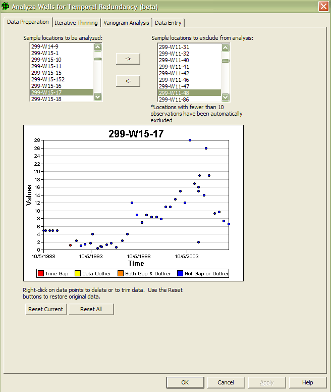
Figure 3.55.  Analyze Wells for Temporal Redundancy Dialog

Step 2 - Choose the type of analysis to perform

As discussed above, the main choice to be made is whether to identify a temporal sampling plan that will allow reproduction of trends seen in the data, or to identify a temporal spacing that should be sufficient to ensure that samples are independent of one another. If the first goal is required, perform iterative thinning, otherwise perform a temporal variogram analysis.

Step 2a - Perform iterative thinning

On the iterative thinning tab, the user first chooses which locations to analyze from the list of available wells. If the user then hits the Calculate button, the iterative thinning is performed for each of the selected wells. The results for each well can be viewed by selecting the well from the list in the Analysis Results.

The display of the results for each well shows the original data, the smoothed curve fit to the data, and a confidence interval around the smoothed curve (Figure 3.56). The default confidence interval is a 90% confidence interval. 

Beneath the graph for each well will be a statement on the original spacing, the optimal spacing based on the parameters that were selected, and the reduction in the percentage of samples that would result at the optimal spacing.

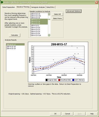
Figure 3.56.  View of Smoothed Curve Fit to a Well's Data

The user can also modify the default parameters used in performing the iterative thinning analysis. By clicking on the Advanced Options button, the user will be presented with the default settings, and can modify them, if desired.

Smoothing bandwidth: Related to the width of the smoothing window used in the Lowess smoother. Default is 0.5, as recommended by Cleveland (1979). Normally set between 0.2 and 0.8. Smaller bandwidths result in less smoothing of the trend, while wider bandwidths result in greater smoothing. The choice of bandwidth should also reflect the amount of data available. Small bandwidths should not be used with sparse time series.

# simulations:  The number of Monte Carlo simulations to perform. In each Monte Carlo simulation a different set of randomly selected samples would be deleted from the base case. The default is 500 simulations. A smaller number would reduce the computational time.

CI confidence: The width of the confidence interval around the smooth trend. Default is set to a 90% confidence interval. The use of a wider confidence interval (e.g., a 95% CI) will make it more likely that the smooth trend fit to a reduced dataset will fall within the chosen CI around the base smooth trend, and thus result in a longer optimal spacing interval. The choice of CI will be documented in the report file.

% of simulated data required within the original trend CI: The default for the percentage of the simulated trend falling within the original trend CI is 75% (Cameron 2004). The choice of a smaller percentage will increase the optimal sample spacing. The percentage chosen will be documented in the report file.

Step 2b - Perform a temporal variogram analysis

The objective of the temporal variogram analysis is to identify the range of the variogram model that best fits the experimental variogram. The model type, nugget, sill and range can all be modified to fit the experimental variogram. If a nested model is required (i.e., one showing multiple structures), the range of interest will be the longest range identified. If an increasing or decreasing trend is present in the concentration data, then the variogram may increase without breaking over into a sill. In that case, the variance of the data can be used to identify the sill that must be reached by the model, so that a range can be identified. The range can then be used as a minimum estimate of the spacing between well samples that would ensure independence of the samples. A brief description of the parameters of the variogram model follow:

Nugget:  Related to the amount of short range variability in the data. Choose a value for the best fit with the first few empirical variogram points. A nugget that's large relative to the sill is problematic and could indicate too much noise and not enough temporal correlation.

Model type: See Deutsch & Journel or Isaaks and Srivastava for the details of these models. Spherical and exponential models are most widely used.

Range: The time after which data are no longer correlated:  approximately the lag spacing where the variogram levels off to the sill.

Sill: The sill is the total variance where the empirical variogram appears to level off, and is the sum of the nugget plus the sills of each nested structure.  Variogram points above the sill indicate negative temporal correlation, while points below the sill indicate positive correlation. The variogram may not exhibit a sill if trends are present in the data.  In that case, one can use the variance of the data as a reasonable default for the sill.

Variogram number: By default a single variogram model is used, but up to three can be nested to more accurately fit a model to the data. In cases where nested scales of temporal continuity appear to be present, it is best to attempt to determine the scientific reason for the multiple nested models (e.g., a short range might be related to daily or other short term variations, with a longer range related to seasonal effects or changes in concentration due to migration of the plume).

For detailed documentation on analyzing redundancy, please refer to the VSP Help Topic Analyze Redundancy.

Previous Next

References