7.0 Unexploded Ordnance Features Within VSP

VSP contains several tools for statistical site characterization protocols of sites potentially contaminated with unexploded ordnance (UXO). These site characterization protocols help identify and delineate potential target areas at a site using limited amounts of geophysical transect data (Hathaway 2008). Tools include approaches for transect design, target identification, boundary delineation, and geophysical anomaly density mapping. The different topics and their corresponding sections in this guide are as follows:

• transect spacing needed to locate target areas (Section 7.1)

• locating and marking target areas based on elevated anomaly density (Section 7.2)

• geostatistical mapping of anomaly density and delineation of target areas (Section 7.3)

• delineating high-density areas (Section 7.4).

• assessing probability of target traversal based on actual transect pattern (Section 7.5)

• post remediation verification sampling (Section 7.6).

7.1 Transect Spacing Needed to Locate Target Areas

For help during this section, please refer to the VSP Help Topic Transect Sampling for UXO Target Detection dialog.

Geophysical surveys are conducted at DoD sites and facilities to search for target areas at which munitions were fired or dropped. Surface areas passed over by geophysical detectors, referred to as transects, are usually up to several meters wide and run in a relatively straight line (as much as terrain permits) from one point of a site to another. When a geophysical sensor system is deployed continuously along transects, anomalies indicating munitions related items may be recorded. A goal of these surveys is to identify areas of high anomaly density consistent with that of a target area. The transect design methods in VSP are statistical approaches for determining the level of confidence in whether a transect sampling design will traverse and/or detect a target area of a specific shape, size, and anomaly density.

Selecting Sampling Goals > Find Target Areas and Analyze Survey Results (UXO) > Transect spacing needed to locate target areas accesses the VSP tools that calculate the probability that at least one transect will traverse a target area of specified size and shape or estimate the probability the target area will be traversed and detected with a specific transect design, assumed background density, and target area density. In addition to these two methods, the user can manually place transects within a sample area.

Table 7.1 lists the variables that can be adjusted in this dialog and identifies which transect design method uses the variable. The three different methods are identified as Traversal, Traversal and Detection, and Manual in Table 7.1. The "additional information" column provides general information about the variable. Each of these variables will be described in more detail in the following sections. The first four variables listed in the table (Transect Pattern, Transect Width, Target Area Shape, Target Area Orientation) are generally defined by the survey equipment and the specific site use. The design objective selected will determine the importance of the remaining variables. The design objectives are specifically stated in VSP as "Ensure High Probability of Traversal Only" (traversal), "Ensure High Probability of Traversal and Detection" (traversal and detection), and "Manual Transect Spacing" (manual).

Of the three transect design methods, the traversal and detection design objective provides the most valuable information about the specific transect design selected. However, as Table 7.1 shows, it requires knowledge and input for many more variables than the other two. The traversal design guarantees that the assumed target area will have a specified probability of being traversed but falls short of any estimate that the target area will actually be identified.

Table 7.1.   Variables That Can Be Adjusted in the "Transect Spacing Needed to Locate a UXO Target Area" Design Dialog with Selected Additional Information About the Variable and If the Variable Is Used in One of the Three Transect Design Methods

7.1.1 Survey and Target Area Pattern

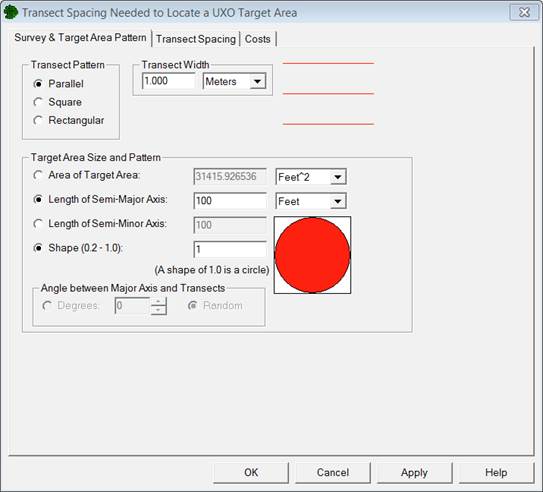
The "Survey and Target Area Pattern" tab shown in Figure 7.1 is used to enter information about the transect pattern of interest, the transect width (width of the area covered by the geophysical detector), the size and shape of the target area, and the angle between the major axis of the target area and the transects.

Figure 7.1.   Survey and Target Area Pattern Tab

7.1.1.1 Transect Pattern

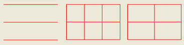
In the example shown in Figure 7.1, a parallel transect pattern has been specified under the "Transect Pattern" section in the upper left corner. In the upper right section, a visual example of the transect pattern is displayed showing three red lines that represent parallel transects.  Figure 7.2 shows the visual examples for all three types of transect patterns: parallel, square, and rectangular.

Figure 7.2.   Transect Patterns:  Parallel (left), Square (middle), and Rectangular (right)

7.1.1.2 Transect Width

The width of the transects is entered under "Transect Width." The transect width, which is dependent on the "sensor footprint," is the width of the area on the ground surface for which the geophysical detector passes over and collects data. Units can be entered in feet, meters, or inches. The transect width along with the transect length determine the amount of surface area a transect covers.

7.1.1.3 Target Size and Pattern

In the "Target Size and Pattern" section of Figure 7.1, different options are available for entering the size and shape of the target area. Options include entering the major axis and minor axis, entering the major axis and shape, or entering the area of the target and shape. There also is an option for fixing the angle of the target in relation to transects or allowing this to be random (the default). The Area of Target Area is the total surface area over which the target area lies. The Semi-Major Axis and Semi-Minor Axis are the widths of the distance from the target area center to its perimeter at its widest and narrowest points, respectively, as illustrated in Figure 7.3. The Shape of the target is the ratio of the semi-minor axis to the semi-major axis. The shape will never be greater than 1 and has a lower-limit of 0.2.

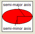
Figure 7.3.  Semi-Major Axis and Semi-Minor Axis on an Ellipse

When the identified target area is not a circle, the angle of orientation between the target area major axis and the transect orientation on the map can be defined or marked as random in the "Angle between Major Axis and Transects" section of Figure 7.1. It is recommended that "Random" be used unless very reliable information is known about the target location and the direction from which the target was fired upon. If this information is available and the angle of the target's semi-major axis is known with near certainty, then "Degrees" may be selected and the angle is entered in degrees. When this information is known, it can have a significant effect on the final transect design.

7.1.2 Transect Spacing

The "Transect Spacing" tab shown in Figure 7.4 is used to enter information about the design objective and parameters needed to assess those objectives other than those covered in the "Survey and Target Area" tab.

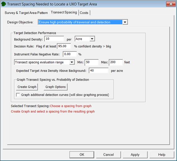
Figure 7.4.   Transect Spacing Tab for Design Objective "Ensure High Probability of Traversal and Detection" and "Transect Spacing Evaluation Range"

7.1.2.1 Design Objective

There are three design objectives to choose from: 1) Ensure high probability of traversal and detection, 2) Ensure high probability of traversal only, and 3) Manual transect spacing.

Figure 7.4 shows the Transect Spacing tab when "Ensure high probability of traversal and detection" is selected as the Design Objective and "transect spacing evaluation range" is selected from the drop-down menu under Target Detection Performance.  Figure 7.5 shows the Transect Spacing tab for the same Design Objective for when "TA density (above background) range" is selected from the drop-down menu.

/p>

Figure 7.5.   Transect Spacing Tab for Design Objective "Ensure High Probability of Traversal and Detection" and "TA Density (above background) Range"

The Background Density of a site is the expected density in an area where anomalies occur solely from geologic material or anthropogenic clutter not related to DoD range activities. These background anomalies are distributed with a consistent background rate throughout the site. Areas containing UXO and other munitions-related anomalies are expected to have density greater than background.

The Decision Rule is the required percent confidence that an area has density greater than background density needed to conclude it is an area of interest  VSP evaluates a number of "windows," which are circular areas centered along transects. The Decision Rule refers to the percent confidence for an individual window. VSP will "flag" an area that appears to have density higher than background density according to the decision rule. An area is flagged if the actual density is significantly higher than the expected background density. In statistical terms, the decision rule is 1 - a expressed as a percentage, where a is the probability of a type I error, or the probability of concluding an area has density greater than background when it is truly a background area.

The Instrument False Negative Rate accounts for the fact that collected data may not be representative of the actual density because the geophysical detector may not identify all detectable anomalies. For example, a false negative rate of 5% would indicate the detector, on average, would fail to detect 5% of the detectable anomalies traversed (background and target area). It is generally assumed that the detector always detects individual anomalies of interest, thus a false negative rate of 0% is used for a default value.

Min and Max refer to a range of transect spacings or target area anomaly densities (above background) to evaluate. When the design objective is Ensure high probability of traversal and detection, the user has the option of choosing to produce a TA density (above background) range or a transect spacing evalu­ation range. When working with a transect spacing evaluation range, users must enter the Min (minimum) and Max (maximum) transect spacings they want to consider. For rectangular transect patterns, this refers to the set of transects with the more narrow transect spacing. Thus, if a user wants to evaluate a range of transect spacings, he would enter this range as the Min and Max. VSP will evaluate the transect spacings Min and Max in addition to spacings between those values. When TA density (above background) range is chosen, Min and Max refer to the target area density above background. VSP will evaluate a range of target area densities above background to estimate how well the transect design will detect the target depending on the anomaly density of that target.

The Expected Target Area Density Above Background in Figure 7.4 is the anomaly density of the target (excluding background density) when transect spacing evaluation range is selected. To evaluate a range of transect spacings, the anomaly density of the target remains fixed. 

The Proposed Evaluation Transect Spacing in Figure 7.5 is the transect spacing to use when TA density (above background) range is selected. To evaluate a range of target densities, the transect spacing remains fixed. Selecting the Graph Additional Detection Curves box works as described in the following paragraph with density and transect spacing interchanged.

Checking the Graph Additional Detection Curves box will produce two additional curves on the graph for the density or transect spacing specified. The additional curves will be for one half and twice the fixed input variable. This allows for the examination of the sensitivity of both changes in transect spacings and changes in target density on the same graph. Because this requires additional simulations for the additional curves, this option increases the simulation run time by a factor of 3.

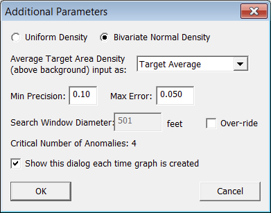
The Graph Options button brings up the additional dialog in Figure 7.6.

The user can choose between a Uniform Density and a Bivariate Normal Density for the distribution of anomalies, excluding background, within the target area. If Uniform Density is chosen, the distribution of anomalies within the target area is assumed to be randomly distributed throughout the entire target area. If Bivariate Normal Density is chosen, the distribution of anomalies within the TA is assumed to be biased toward higher densities in the center of the TA such that the densities from the TA center to the TA perimeter follow an approximately normal curve.

Average Target Area Density (above background) defines how the density value inputs for the Bivariate Normal Density are entered when selected (this option is disabled when Uniform Density is selected). The default is that target area densities are entered as the Target Average, or average anomaly density (above background) of the target. Also available are Outer Edge of Target and Center of Target, which refer to the density near the perimeter of the target area and the center of the target area, respectively. Changing to one of these options will allow the user to enter target area densities for the target edge or center instead of the target area average anomaly density.

Min (Minimum) Precision is used to determine the number of different TA densities or transect spacings to simulate. Decreasing the Min Precision typically requires more transect spacings or densities to be simulated and increases the length of the simulation. Increasing the Min Precision will typically decrease the length of the simulation.

Max (Maximum) Error determines the number of iterations for each transect spacing or density simulated. Decreasing the Max Error requires more simulations for each transect spacing or density simulated and increases the overall simulation time. Increasing the Max Error will decrease the simulation time.

The Search Window Diameter refers to the diameter of the circular search window used to identify areas in which density is greater than background density. The window is actually a moving window that moves in increments of one-sixth the window diameter along each transect, as shown in Figure 7.7. Each search window is evaluated to determine if the density is significantly greater than background density. VSP calculates a default window diameter for the current design, but checking the Override box allows the user to manually enter a window diameter. The Critical Number of Anomalies refers to the number of detected anomalies required inside a window to identify it as significantly greater than background.

Checking the Show this dialog each time graph is created has the dialog box in Figure 7.6 appear after pressing the Create Graph button (Figure 7.4 and Figure 7.5) but before simulations are run and a graph is produced. Otherwise, pressing the Create Graph button will skip this step and proceed with running simulations followed by producing a graph.

An example of the resulting graph, or power curve, for this tool is shown in Figure 7.8, where Transect spacing evaluation range was selected and the Graph Additional Detection Curves box was checked. This graph shows the effectiveness of a range of transect spacings for detecting the target area. It also shows the sensitivity of detecting the target area for different target area densities.

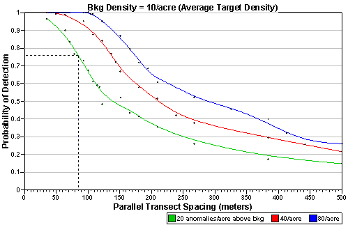
Figure 7.8.   Power Curve with Transect Spacing as the X-Axis and Additional Curves Displayed

Figure 7.9 shows the Transect Spacing tab when "Ensure high probability of traversal only" is selected as the Design Objective. A subset of the parameters used for "Ensure high probability of traversal and detection" is used for this dialog with one new parameter, Required Probability of Traversing the Target. This is the required probability the design chosen will traverse the target area. VSP calculates the transect spacing required to achieve this probability and displays the result in red text. These parameters allow the user to specify the Target Area Density Evaluation Range to examine how well the transect design will detect the target area for different target area densities. 

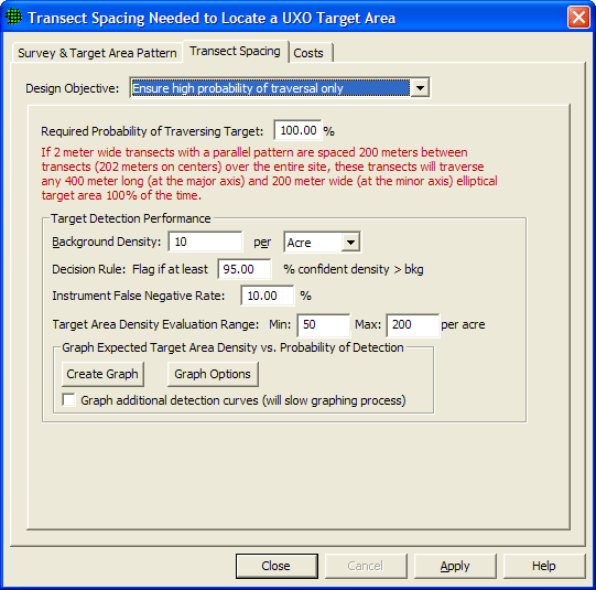
Figure 7.9.   Transect Spacing Tab for Design Objective "Ensure High Probability of Traversal Only"

Figure 7.10 shows the Transect Spacing tab when "Manual transect spacing" is selected as the Design Objective. This option makes available some of VSP's useful features without using data quality objectives. Before deciding to develop a sampling plan based on a user-supplied transect spacing and starting location, consider the assumptions and limitations involved.

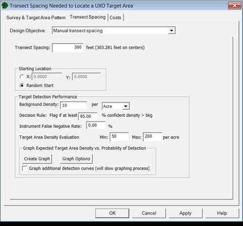
Figure 7.10. Transect Spacing Tab for Design Objective "Manual Transect Spacing"

7.1.3 Costs

The Costs tab provides an estimate of costs using the chosen transect design on the current VSP map. The user must enter the Fixed Planning and Validation Costs, Setup Cost per Transect, and Collection Cost per Linear Unit to calculate the Total Cost of Transect Sampling.

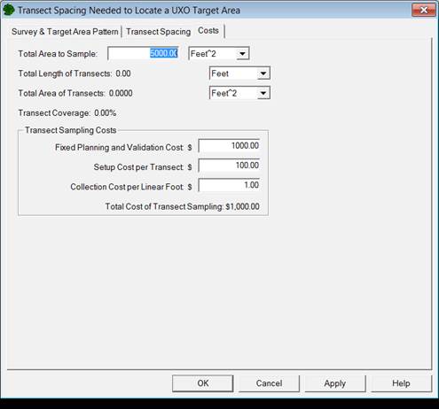
Figure 7.11. Costs Tab for Transect Spacing Needed to Locate a UXO Target Area

7.2 Locate and Mark UXO Target Areas Based on Elevated Anomaly Density

Once a transect design has been accepted and the geophysical survey completed, the surveyed data (i.e., the transect course-over-ground and anomaly location data) is imported into VSP and analyzed.  This process is begun in VSP by selecting Sampling Goals > Find Target Areas and Analyze Survey Results (UXO) > Locate and mark target areas based on elevated anomaly density.  Section 7.2.1 details how these data can be imported and manipulated in VSP. Section 7.2.2 describes the methods used to evaluate the anomaly density distribution of the site and determine an appropriate critical density to identify high-density areas within it. 

7.2.1 Data Entry - Importing Course-Over-Ground and Anomaly Files into VSP

For help during this section, please refer to the VSP Help Topic UXO Data Entry Sub-page.

The Data Entry tab shown in Figure 7.12 provides the ability to import ASCII (plain text) files identifying the course-over-ground (COG) and anomalies (anomaly) data. Table 7.2 shows an example of the COG file (left) and anomaly file (right) structure used within VSP. Oasis Montaj can be used to generate COG and anomaly files like those shown in Table 7.2 (Geosoft 2007). VSP can also import the COG and anomaly information if they are saved in common TXT and CSV formats. The two files shown in Table 7.2 show the most information that can be included in the file. At a minimum, the file to be imported must have two columns representing the X and Y coordinates in that order. The COG coordinates mark the X, Y location for the survey equipment path. Because the file does not provide transect width information, the user must obtain it from the survey team. The anomaly coordinates are locations where the survey team has identified an object of possible metallic origin.

Table 7.2.   Example of ASCII Files That Can Be Imported into VSP for the Course-Over-Ground Transect Data and the Associated Anomaly Location Data

The Data Entry dialog in VSP provides the user with the ability to import and identify all the necessary files for analysis. Figure 7.12 shows the "Data Entry" sub-tab (left) and the "Plots" sub-tab (right) included in the "Locate and mark UXO target areas based on elevated anomaly density" and "Geostatistical mapping of anomaly density" dialogs under the "Data Entry/Plots" tab. The "Data Entry" sub-tab provides import, export, removal, and file summaries for the COG and anomaly files in two separate boxes. When importing COG information, the user is prompted to define the width of the transects in the file before it is imported. VSP provides a summary that includes the file name, number of lines imported, width of the transects, and the units associated with the transect width. The anomaly data is imported and summarized in a similar manner. The "Selected" column shown in each box provides a method to manipulate individual files. If the box is blank, the file is not selected. When the user checks the box, then the identified files can be removed or exported from the project. If the box is checked next to "Mark points that are outside Sample Areas," then any points in an imported file that fall outside the selected sample areas are shown as red points. This feature helps the user identify locations where the survey went beyond the identified sample boundaries. The "Plots" sub-tab shows plots of the data resulting from the "Find Target Areas" tab that is explained in the following section.

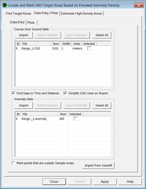
Figure 7.12. Data Entry Tab Found Within the "Find UXO Target Areas" Dialog and "Geostatistical Mapping of Anomaly Density" Dialog

7.2.2 Find Target Areas

After the sample area has been identified and the necessary files have been imported into VSP, the user can analyze the data. VSP provides two dialogs for analyzing the spatial data. This section details the dialog of the "Find Target Areas" tab when selecting Sampling Goals > Find Target Areas and Analyze Survey Results (UXO) > Locate and mark target areas based on elevated anomaly density. This identifies locations within the transects that are identified as being high density (i.e., high number of anomalies within a specified amount of the surveyed transect area). The dialog for geostatistical methods is discussed in Section 7.3.

To identify high-density areas along transects, VSP passes a circular window over segments of the site and calculates the anomaly density for each window. The Window Diameter specifies the size of the circular area over which the average density is computed. This window diameter was previously explained in Section 7.1.2.1 when describing the Search Window Diameter and the associated search window. The dialog on the left in Figure 7.13 shows where the window diameter is selected in this VSP analysis dialog and the dialog on the left is the window that is displayed upon clicking Help me choose window size that can be used to provide a visual evaluation of appropriate window sizes which will be explained in more detail later in this section. Figure 7.14 provides an example of how the window diameter is used to calculate transect grid densities. The window diameter defines the size of a centered circular window (purple and pink circles in Figure 7.14), which moves every one-sixth the selected diameter and uses the anomaly count with the transect area within the window to calculate a density assigned to the central transect grid (purple and pink boxes in Figure 7.14) centered in the window. The green dots in Figure 7.14 represent the identified anomalies within the two surveyed transects. For transects with length less than one-sixth the window diameter, such as in course-over-ground data, the window may step over several transects.

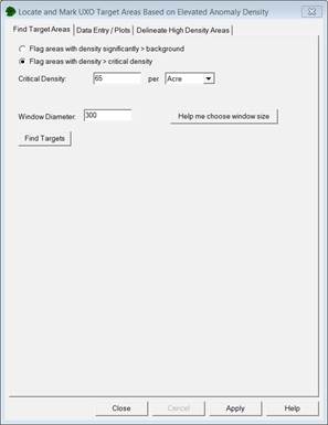
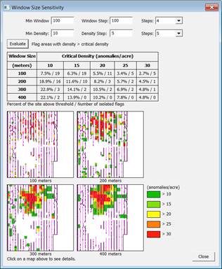
Figure 7.13. Find Target Areas tab when "Flag Areas with Density Significantly
 > critical density" is selected (left) and the results from using the "Window Size Sensitivity" dialog (right) that appears when pressing the button Help me choose window size.

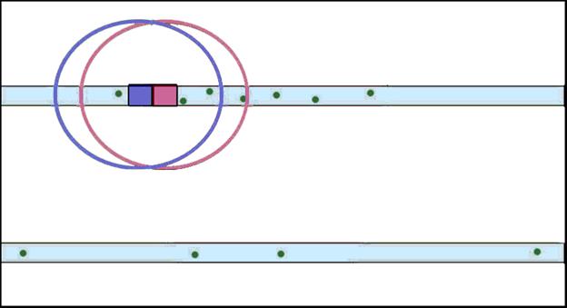
Figure 7.14. Depiction of the Window Density Calculation Process Used To Identify High-Density Regions Within a Site

The selection of an appropriate window diameter is dependent on the size of the target area of interest, transect width, and spacing between transects. The optimum window diameter is one that has sufficient traversed area within the window without including such a large area that potential high-density areas can be masked by the surrounding low-density areas in the window. As a general rule, the window diameter should be less than the diameter of the target area of interest and no smaller than the spacing between the original transect design. Selecting the appropriate window diameter for each specific site analysis is currently left to the user.

A circular search window is used to identify areas in which density is significantly greater than background density or greater than the critical density. The diameter of this window is entered as a parameter in the units to which the VSP map is set. The window is actually a moving window that moves in increments of one-sixth the window diameter along the transect path. Each search window will be evaluated to determine if the density is significantly greater than background density or greater than the critical density, depending on which option is chosen.

Figure 7.13 shows the dialog box when Flag areas with density significantly > critical density is chosen. The Window Diameter and Critical Density are entered and VSP will flag any window whose calculated anomaly density is greater than the specified Critical Density.

The other option is Flag areas with density significantly > background.  This option performs a statistical test on each window to determine if the anomaly density in the window is significantly greater than background density. In addition to the Window Diameter, the user must enter the Background Density and Required Confidence Window Density > Bkg (Background Density). These parameters were previously defined as Background Density and the Decision Rule used in Section 7.1.2.1.

When the Find Targets button is pushed, areas with high densities according to the inputs described above are flagged (marked with a box) on the VSP map. VSP also provides a histogram of anomaly densities across the site created by gridding the site, averaging the window densities in each grid, and displaying these averages in the histogram. This averaging ensures that areas of the site containing more transects will not be overrepresented in the histogram. A histogram of the density calculations for the entire site can provide a good understanding of the anomaly density distribution and can help in selecting the background density. Examples of three histograms are shown in Figure 7.15. The topmost histogram shows

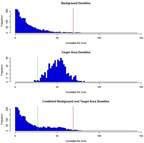
Figure 7.15. Distribution of Background Densities with Average Density of 15 ApA (anomalies per acre) and Standard Deviation of 15 ApA (top); (middle) Distribution of Target Area densities with Average Density of 50 ApA and Standard Deviation of 10 ApA; (bottom) Sample Distribution of Combined Density Distribu­tion. The green line at 27 ApA is the point at which 99 percent of the target area densities are larger. The red line at 70 ApA is the point at which 99 percent of the background densities are smaller.

the distribution of densities in background areas on the site (areas not contained within a target area). The middle histogram shows the densities from a target area. The bottom histogram shows the combined densities from the first two. The bottom histogram is an example of a histogram produced in VSP where densities associated with the target area cannot be deciphered. The VSP user typically will have to try different combina­tions of parameters (i.e. window size and critical density) and use the spatial map of "flagged" regions to get a feel for where possible target areas may lie and to get an idea of the site's possible background density.

The Help me choose window size button shown in left dialog in Figure 7.13 provides the VSP user with the ability to visually evaluate and compare multiple combinations of window sizes and critical densities. The result of one of these evaluations is shown on the right in Figure 7.13. Before the map and table are displayed the user must identify the different window size and critical density combination they would like to evaluate. This is done by selecting the minimum window size (Min Window), minimum critical density (Min Density), step size (Window Step and Density Step), and number of steps (Steps:) for evaluation. With these inputs selected the VSP user can then press the Evaluate button. The table and individual "flagged" maps allow the user to evaluate the sensitivity to different combinations of window size and critical density.

7.3 Geostatistical Mapping of Anomaly Density

Within VSP, the geostatistical anomaly density mapping is composed of two primary tasks. The first task is to model the spatial variability of the measured anomaly densities as determined from the geophysical transect data. This task involves the development of a variogram based on the window-averaged transect density values.  A variogram depicts how the variability of a set of values changes as the distance between the spatial locations of these values increases. The second task involves the estimation of anomaly density at unsampled locations within the study area through a geostatistical methodology known as kriging. Kriging uses the model of spatial variation as captured by the variogram to provide an unbiased, minimum-variance estimate of the anomaly density. Kriging is the procedure that creates the final anomaly density map. To use these methods, GAM/GAMV and KT3D also must be installed (see vsp.pnl.gov).

An anomaly density map can be created from the sample transect data by opening the "Geostatistical mapping of anomaly density" dialog (Figure 7.16). This dialog is opened by selecting "Sampling Goals > Find Target Areas and Analyze Survey Results (UXO) > Geostatistical Mapping of Anomaly Density". This selection presents a menu with four screen tabs. The default tab, "Map Anomaly Density," presents several options for mapping anomaly densities. The second tab, "Variogram Model," provides an alternate means of accessing variogram fitting parameters once the variogram has been computed. The third tab, "Data Entry and Analysis," provides the ability to import files identifying the course over ground and anomalies as explained in Section 7.2.1. The fourth tab "Delineate High Density Areas" contains tools used in locating target area locations based on anomaly density values. These tools are explained in Section 7.4.

There are two pathways to creating the anomaly density estimates. The basic pathway will create an estimate of anomaly density based on a series of default values computed from the current data set. The advanced pathway allows more control over the variogram and kriging parameters, but requires the user to possess a greater understanding of geostatistical analysis to be used in a meaningful manner. Each of these pathways is discussed below.

7.3.1 Basic Geostatistical Mapping

Under the default "Map Anomaly Density" tab of the "Geostatistical Mapping of Anomaly Density" dialog, the user is presented with two choices for computing the anomaly density map. In "Basic Mode," VSP will automatically compute a variogram and perform the kriging necessary to develop a spatial estimate of anomaly density. In this mode, a series of default values is computed for the data set and used in the variogram and kriging analyses. This mode is fully automatic and is the recommended path for new users to follow.

Figure 7.16. "Geostatistical Mapping of Anomaly Density" Dialog.  This view shows the basic mode without the advanced operations screen box displayed.

To use the automatic mode, click on the "Launch" button within the "Basic Mode" screen box (Figure 7.16). Clicking on this button will launch a series of programs that will momentarily flash several operational windows to the screen before returning to the "Geostatistical Mapping of Anomaly Density" dialog. After successful completion of this process, the modeled variogram can be viewed by clicking on the "Variogram Model" tab in the "Geostatistical Mapping of Anomaly Density" dialog. Clicking on the "OK" button will close this dialog and load the anomaly density estimate map as an overlay onto the main VSP site map. Clicking on the "Apply" button will load the results into VSP but keep the geostatistical mapping window open. At this point, the primary VSP mapping tools can be used to investigate the details of the estimated anomaly density map.

7.3.2 Advanced Mode Geostatistical Mapping

In the "Advanced" mode, the user is given complete control over all the parameter settings involved in the variogram and kriging analysis. This mode is recommended for experienced users or when specific analysis parameters are necessary.

Advanced mode is selected by clicking on the "Advanced" button under the "Map Anomaly Density" tab of the "Geostatistical Mapping of Anomaly Density" dialog. Clicking on this button will open a screen box with various selections for advanced mode operation (Figure 7.17). One parameter setting is directly available from this screen box. This is the averaging window diameter. This value specifies the size of the averaging window for computing the anomaly density values used in the geostatistical mapping. The variogram lag distance and kriging grid cell size also are affected by this parameter. The lag distance is the separation distance between pairs of data points. The lag distance collects the data pairs into groups based on separation distance and is discussed further below. The initial lag spacing and kriging grid cell size are set to be one-sixth the averaging window diameter by default. If an averaging window diameter other than the default value is desired, it should be changed before proceeding with the next steps in the analysis. The initial lag spacing and kriging grid cell size also can be changed by manually entering them using the advanced mode.

The first processing step in the "Advanced Mode" is to click on the button labeled "GAM/GAMV." This selection will initiate the variogram calculation and then open a separate screen presenting a graphical interface for additional variogram analysis. At this point, the automatically fit variogram model can be viewed by clicking on the "Fitting" tab of the GAM/GAMV" screen (Figure 7.18). Here, the user will see the empirical variogram values as well as the automatically fit variogram model and its parameters (Figure 7.19). The variogram is computed from the averaged anomaly density values obtained from the geophysical survey transect data. The averaged anomaly densities are computed automatically using the averaging window diameter specified under the "Advanced Options" screen box, and the previously loaded anomaly locations and course over ground information. These values are then passed automatically to the GAM/GAMV code.

The "Variogram Control Parameters" tab in the GAM/GAMV screen provides access to other variogram analysis parameters. Details regarding these other input parameters are given in GAM/GAMV interface code help files, and a full discussion can be found in Deutsch and Journel (1998). In general, the only control parameters that might typically be altered at this stage in the analysis are the lag spacing, lag tolerance, and number of lags to compute. These parameters control how the observations for computing the empirical variogram are grouped and the maximum separation distance that should be considered. These parameters are discussed further below.

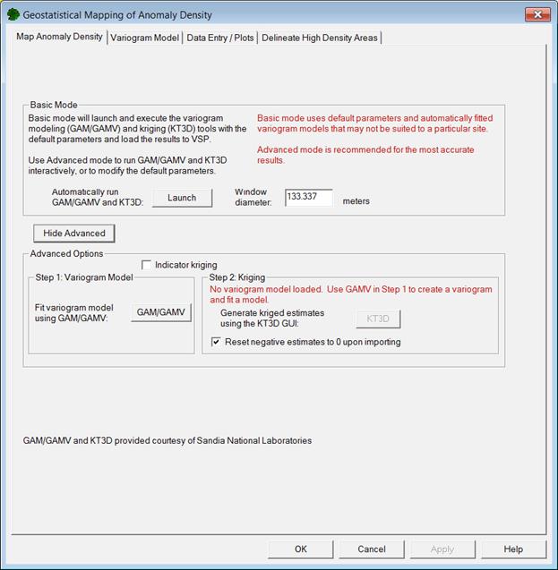
Figure 7.17. Advanced Mode for Geostatistical Anomaly Density Mapping

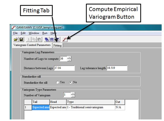
Figure 7.18.    Aspects of the GAM/GAMV Interface Screen

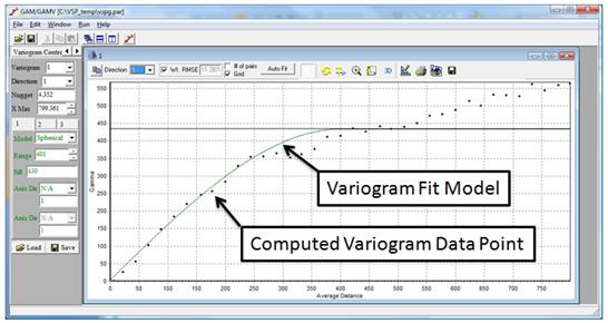
Figure 7.19. Variogram Fitting Screen from the GAM/GAMV Window.  Dots show computed variogram values, and the solid green line shows the model fitted to variogram values.  Parameters for this model are listed along the left side of the window.

The GAM/GAMV code is used to compute a variogram for the averaged anomaly density data. A variogram depicts how much the variation between pairs of sample values (anomaly density in the case here) changes as the distance between pairs increases. The lag distance-the separation distance between pairs of data points-is used to group the data pairs into groups based on separation distance. Then the "semi-variance" is computed for each group and plotted as part of the empirical variogram. Because most sample points will not be separated by exactly the specified lag distance, the lag tolerance is given to include those observations that are within the tolerance value of the specified lag distance. For example, using a lag distance and tolerance of 200 m and 100 m, respectively, will generate the following grouping of separation distances:

0 to 100 m                           group 1

100 to 300 m                       group 2

300 to 500 m                       group 3

A semi-variance value for each group is then computed using all the data points with separation distances falling within the distance boundaries for that group. The separation distances are simply the straight-line distances between the sample pairs based on the sample point locations. The semi-variance values are computed using the equation shown below. In this equation h is the lag distance, Z(x_i) is the value of our variable (anomaly density) at a given location, n is the total number of sample values, and \(\gamma\) is the computed semi-variance value at that lag distance. The computed semi-variance values are then plotted along with the average separation distances for each group to create an empirical variogram (Figure 7.19). The empirical variogram is a graph showing one-half the average squared differences between all observations for a series of average lag distances.

$$ \gamma (h) = \frac{1}{2n} \displaystyle\sum_{i=1}^n (Z(x_i) - Z(x_i + h))^2 $$

The solid dots in Figure 7.19 show the computed experimental variogram values for specific lag distances. The X-axis shows the lag distance in length units (meters in this case), and the Y-axis shows the computed semi-variance value.  In this example, the lag distance was 200 m and the lag tolerance was 100 m. The actual location of each data point on the X-axis is determined by the average actual lag distance of all the data pairs in that group. The solid green line shows the automatically fit variogram model for this data set.

One-half the average squared difference for all of the pairs of observations for each lag group will show up as a single data point on the experimental variogram. Within VSP, the along-transect data point spacing is controlled to be one-sixth the averaging window diameter; this is typically the minimum lag distance that should be used. This minimum value is a good place to start the variogram analysis and typically is sufficient for most studies. To include all data points and avoid overlap between variogram point groups, the lag tolerance should be set to one-half the lag distance. After any of the GAM/GAMV input parameters are changed, the variogram will need to be recomputed by clicking on the "Compute Empirical Variogram" button (Figure 7.18). This selection will recalculate the empirical variogram and display the results under the "Fitting" tab.

The "Fitting" tab of the GAM/GAMV window (Figure 7.18) interface will display the computed empirical variogram, and will also automatically compute an initial model to fit the data points. This model consists of a continuous function that closely matches the distribution of the empirical variogram data points. A continuous function that will produce a positive definite covariance matrix for solving the kriging equations is required as a model of spatial variability. Although a single model typically is sufficient, up to three different models can be nested simultaneously to provide a proper fit to the empirical data points. Excessive time should not be spent in creating a best-fit model of the empirical variogram data. Typically, the focus of the variogram model fitting should be on matching the experimental variogram points at the shorter lag spacings; the variance of the data set, shown by the solid horizontal black line, provides the theoretical maximum variogram value (see Figure 7.20). A reasonably good fit is usually sufficient when using sample transect data set.

The variogram model is reshaped by changing the range and sill values (Figure 7.20). The sill controls the height of the variogram model while the range controls the distance scale of the model. If a large initial jump in the variance is needed to match the empirical data, the nugget value can be increased. The nugget, sill, and range can be adjusted to match the computed variogram data points as needed. In addition, the basic model type (e.g., spherical, Gaussian, exponential) also can be changed as needed. The variogram model line will change dynamically as any of the modeling parameters are altered.

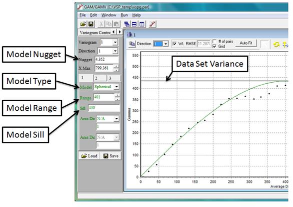
Figure 7.20. Variogram model parameters settings within the GAM/GAMV Graphical Interface

Figure 7.21 shows the effects of changing the range and sill values of the variogram model. The sample data for these plots were from a magnetometer survey of a portion of the Pueblo Precision Bombing Range in southeastern Colorado. The magnetometer transects from this survey were nominally spaced at 155 m and crossed two large high-density areas. As shown in these plots, the range and sill values can be adjusted until a sufficiently close match to the empirical data is made.

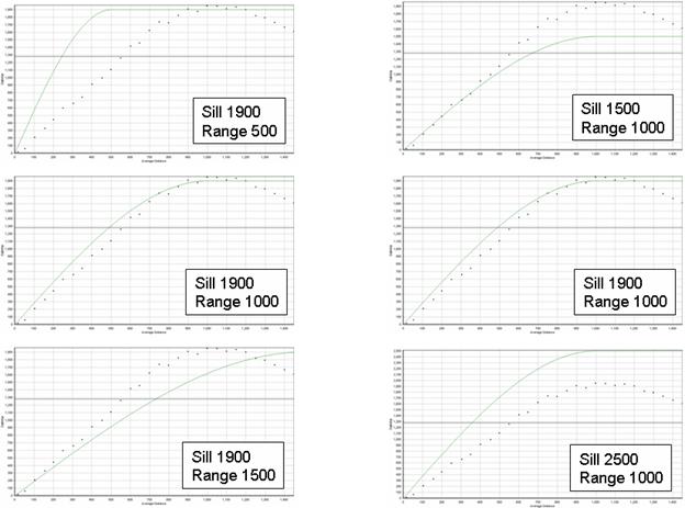
Figure 7.21. Effects of Changing Sill and Range Values for Variogram Model.  Left column of plots shows effects of altering range value; right column shows effects of altering sill value.  In each plot, dots represent empirical variogram values, and the green line shows model variogram.

Once the variogram model is fit satisfactorily, the GAM/GAMV interface can be closed. The next step is to create a map of the anomaly density across the site using the information in the variogram model. The spatial estimation tool is "KT3D." To begin, click on the KT3D button within the "Geostatistical Mapping of Anomaly Density" dialog.  This will open the KT3D graphical user interface. The variogram model parameters developed using GAM/GAMV will be passed automatically to KT3D.

The KT3D interface provides control of several parameters for the KT3D kriging code. A number of default parameters are already set, so the code can be run immediately by clicking on the "Run" button (Figure 7.22).  This will generate a kriging estimate of anomaly density and display the results within the KT3D interface screen. To display the kriged estimate within VSP, simply close the KT3D interface screen, then click "OK" or "Apply" within the "Geostatistical Mapping of Anomaly Density" dialog box.

The other advanced options for running KT3D can be accessed through the various tabs under the main "Parameters" tab on the interface screen. A complete explanation of these various options is presented in the associated help files contained within the KT3D tool. 

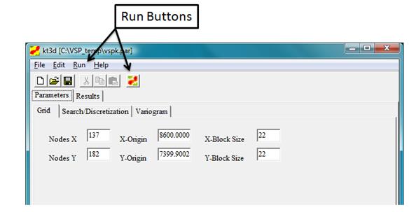
Figure 7.22.  KT3D Interface Screen

The KT3D parameters most likely to be changed from their defaults are the gridding and search parameters. These parameters, which control the number, size, and extent of the estimation cells used to discretize the site and the search of local data to be used in the estimation of any location, respectively, are located under the "Grid" and "Search/Discretization" tabs. 

Typically, the default values for these parameters are sufficient and appropriate. These parameters are explained fully in help files associated with the KT3D program, and a full discussion of the background of the estimation can be found in Deutsch and Journel (1998). It is important to remember that the X and Y node count and X and Y block sizes are used in conjunction to determine the area covered by the kriging estimation; changing one without changing the other may result in a kriging estimation area which is smaller or larger than your original transect sampling domain.

After all the parameters are set, the user clicks on the "Run" button to run KT3D. The kriging results are displayed automatically within the KT3D interface sub-window. In addition to the anomaly density estimate, the kriging variance is displayed in an adjacent window. Closing the KT3D interface window will return the user to VSP and the "Map Anomaly Density" dialog. Clicking on "OK" or "Apply" will display the kriging results in the VSP display.

7.3.3 Display of Kriging Results Within VSP

For help during this section, please refer to the VSP Help Topic Geostatistical Mapping of Anomaly Density Dialog.

Whether run from "Basic" or "Advanced" mode, clicking on the "Apply" or "OK" button in the "Map Anomaly Density" screen will display the current kriging results within the VSP mapping window. The anomaly density map is displayed in VSP as a color-shaded value map. Figure 7.23 shows kriging results displayed in VSP. The anomaly density estimate in Figure 7.23 was developed from magnetometer surveys from a portion of the Pueblo Precision Bombing Range. The site is a World War II-era bombing range that shows evidence of two large target areas. The default color scheme in the map display shows the highest density values in red and the lowest values in green.  A color scale is provided to aid in interpretation of the results. The lack of color shading (background color is displayed) indicates that no kriging estimation was performed for that location. This typically is the result of a lack of enough sample transect data within the search window for reliable estimates within that area.  An example of this

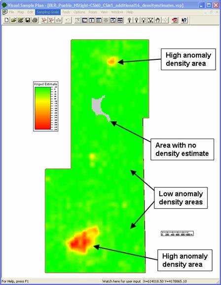
Figure 7.23. Results of Kriging Estimation Displayed in VSP

can be seen in Figure 7.24 as a gray area in the northern portion of the study area. Transects were not surveyed in this area because of vegetation and terrain issues. Because of this gap, no kriging estimates were developed for this area.

During examination of the anomaly density map, it is useful to turn on the display of the transect survey traces and the detected anomaly locations as aids in interpreting the anomaly density map (Figure 7.24). The controls for turning different map elements on and off are located under the "View" menu, or in the "Layer Control" side bar of the main VSP screen. These provide a listing of different mapping elements that can be checked on or off to control the display. The transect survey and detected anomaly locations provide a visual relationship between the kriging results and the support data used in the kriging analysis. For example, the transect traces shown in Figure 7.24 explain the gap in the kriging results in the northern portion of the Pueblo Precision Bombing Range study area.

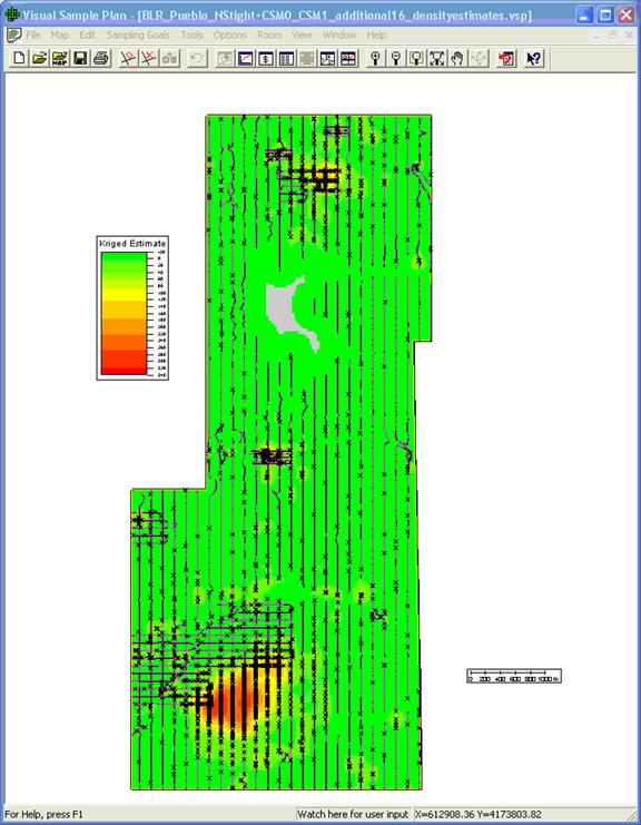
Figure 7.24. Results of Kriging Estimation Displayed in VSP Along with Course-over-Ground Traces and Anomaly Locations

The color scheme used for the anomaly density display can be changed by selecting the "View" pull-down menu on the main VSP screen, then choosing "Kriged Data" and selecting "Color Options." Various color palettes are available. Selecting one with a larger color range will bring out more details in the anomaly density estimate. Figure 7.25 shows the same anomaly density estimate for the Pueblo Precision Bombing Range as shown in Figure 7.23, but a different color palette (MBCGYOR-Grad) is used to enhance the variations in anomaly densities, thus bringing out some of the subtle details in the higher-density areas.

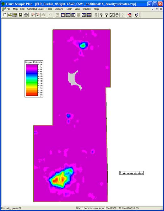
Figure 7.25. Kriging Results Displayed in VSP Using an Alternative Color Scheme

In addition to the estimate of anomaly density, the kriging procedure generates a map of the estimation variance. Figure 7.26 shows the kriging estimation variance computed for the kriging results from the Pueblo Precision Bombing Range study area. The estimation variance shows the uncertainty of the kriging estimate and is a function of the data configuration and the variogram model. Estimates of anomaly density for locations on or near sample transects should be very accurate and, hence, have a low uncertainty. Conversely, estimates distant from the sample transects are likely to be less accurate with a relatively high uncertainty. The value of the estimation variance reaches a maximum at distances greater than or equal to the variogram range away from the nearest data point. The map of estimation variance shows how the variance of the anomaly density changes across the study site. In Figure 7.26, the highest variance values are shown in shades of red; the lowest values in shades of green.  The highest variance values occur in the northern portion of the site where there is a large gap in the sample transects because of terrain and vegetation issues. The maximum variances occur on the edge of the region where no estimates could be made. These high variance values indicate that some areas exist within the site where there are enough nearby data points to create a kriging estimate, but the uncertainty in these estimates is large. While not explored further here, the kriging variance provides a means of identifying regions of high uncertainty and can be used to design additional transect surveys. The lowest variance values are found at the survey transect locations.

The anomaly density estimates can be exported to a file format that is compatible with the ESRI ArcGIS geographic information software system. This is done by selecting "Map > Export" from the main VSP screen. This will provide options for exporting the current kriging estimates or the kriging variances. Maintaining the filename extension of "ASC" will provide direct recognition of the export file within ArcGIS. This export file format can be read directly into ArcGIS.

To view the estimation variance, select the "View" pull-down menu on the main VSP screen, then choose "Kriged Data" and select "Kriging Variance." As shown in Figure 7.26, there is a strong relationship between the sample transect locations and the kriging variance. The variance is lowest near the transects and increases with increasing distance from the sample locations. This can be used as a quick check to confirm that all the appropriate sample data have been included in the kriging analysis and to identify areas where the confidence in the kriging results could be increased with additional sample data.

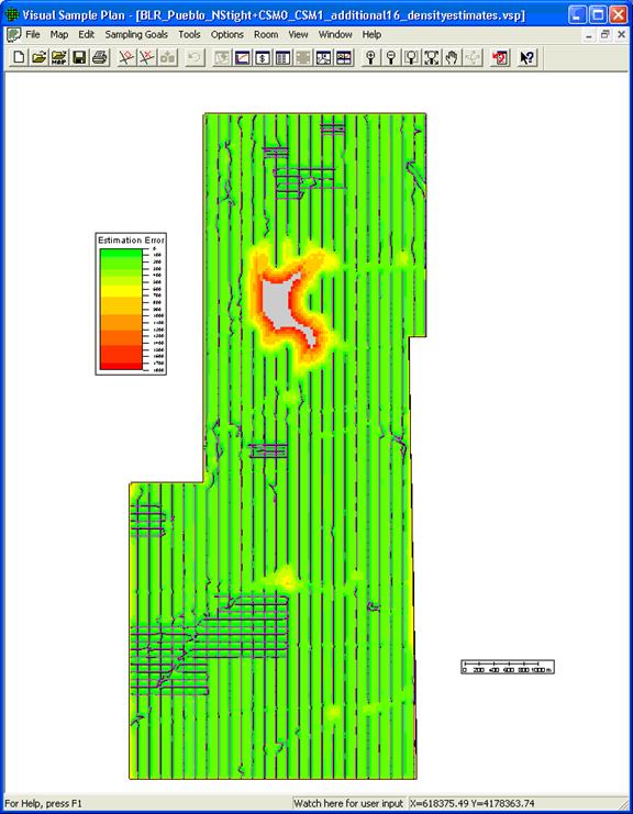
Figure 7.26. Kriging Variance Displayed in VSP Along with Course-over-Ground Traces. The highest variance values are shown in red, the lowest values in green.

7.4 Delineating High-Density Areas

For help during this section, please refer to the VSP Help Topic UXO: Delineate High Density Areas Tools.

Tools for delineating high anomaly density areas can be found under the "Delineate High Density Areas" tab of both the flagging menu window and the geostatistical mapping menu window. These can be accessed by selecting Sampling Goals > Find Target Areas and Analyze Survey Results (UXO) > Locate and mark target areas based on elevated anomaly density or, Sampling Goals > Find Target Areas and Analyze Survey Results (UXO) > Geostatistical Mapping of Anomaly Density from the VSP menu. Figure 7.27 shows the high density area delineation window when accessed from the "Locate and mark target areas..." window. This window contains selection buttons for activating the delineation tools and a table listing the results of the delineation process.

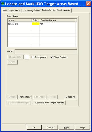
Figure 7.27.  Delineation window.

7.4.1 Delineation from Target Flagging Results

To use the delineation tool based on transect flagging results, the flagging must be performed prior to using the delineation tool. When the "Automatic from Target Markers" button is selected, the window shown in Figure 7.28 is displayed. This window lists the parameters for delineation using the results from target area flagging. 

Figure 7.28. Target area delineation parameters

The parameters for high anomaly density (target) area delineation based on flagging results consist of the block size to put around each marker flag and the minimum size of a high density area to be considered for delineation.  The block size parameter specifies the XY extent of the area around each flagged high density location to be included in the designation of a target area.  It is important that this value be slightly larger than the transect sample spacing in order for adjacent transects to be grouped together into a common target area.  If this value is too small, then adjacent transects with high density locations will be marked as individual target locations instead of being grouped together.

The Minimum size of target area specifies a size threshold below which a delineated area is considered too small to be a valid target feature.  All delineated areas below this threshold are dropped from the listing of delineated areas and not added to the table of potential target areas.  Be sure to choose appropriated units for this value. For reference, the parameters window provides the diameter of a circle of the minimum target area size.

Once the appropriate values for all the parameters are set the "OK" button can be clicked.  This will run the target area delineation and present the results in a table as shown in Figure 7.29.  The table in the upper portion of this window lists all the high density areas delineated for the active sample areas.  Each entry is color coded with a color which correlates to the colored regions shown on the map view (Figure 7.30).

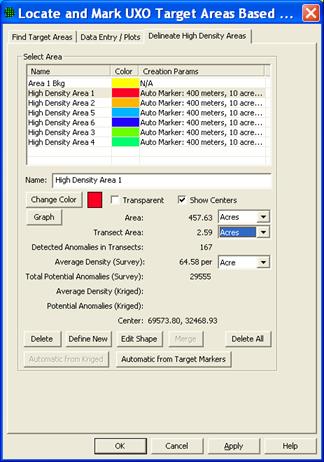
Figure 7.29. Results from high density area delineation tool.

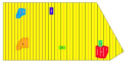
Figure 7.30.  Delineated target areas shown in map view.

When each delineated target area row in the table is selected, the spatial statistics for that delineated area are displayed in the window. These include the total area, total transect length falling within, total number of anomalies, etc. for that delineated area.

The "Change Color" button allows you to customize the color used for each delineated area. The "Graph" button will plot a histogram or box-and-whiskers plot for the selected delineated area. The "Name" text box allows you to change the text name associated with each delineated area. The "Transparent" check box replaces the color fill for the delineated areas with a colored polygon outline and the "Show Centers" check box places a circle with cross-hairs symbol at the center of each delineated area.

In addition, the lower portion of the window displays buttons to delete individual areas, manually define new areas by drawing a polygon, edit the shape of an existing area, or merge two adjacent areas. Any modifications to a delineated area will be recorded for that area and displayed in the table listing. The "Delete All" button will delete all the delineated areas. This is very useful when investigating different delineation threshold values in an iterative fashion.

7.4.2 Delineation from Geostatistical Estimation of Anomaly Density Results

The process for delineating high density areas based on the results of geostatistical estimation is very similar to that used for the flagging results. The geostatistical estimation of anomaly density must be completed prior to using the delineation tool. 

For delineating areas based on the results from geostatistical estimation, the delineation window is accessed as described above and can be found either from the flagging window or the geostatistical estimation window. If a kriged estimate of anomaly density is available, then the "Automatic from Kriged" button will be active. Clicking on this button will bring up the "Parameters for Target Delineation" window as shown in Figure 7.31. There are two parameters which may be set from this window. The minimum target area size parameter controls the smallest region considered as a valid target area. This is the same parameter as was described under the delineation from flagging results procedure. The minimum kriged value specifies the threshold for delineating a target area. Regions with anomaly densities at or above this threshold will be delineated as a potential target area if they meet the minimum size criteria. Once the parameters are set, clicking on the "OK" button will run the delineation process and display the results in a window similar to that shown in Figure 7.29.

All the other options for investigating and interacting with the delineated target areas described under the flagging delineation also apply to the results from the geostatistical estimation delineation.

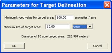
Figure 7.31.  Parameters for target area delineation using geostatistical anomaly density estimates.

7.4.3 Plotting Results from Delineation

Comparative plots of the anomaly density values for the different delineated areas can be viewed by clicking on the "Data Entry/Plots" tab, then selecting the "Plots" sub-tab (Figure 7.32).  This sub-tab provides access to color-coded histograms and box-and-whisker plots comparing the anomaly density values of the various delineated areas and background (shown in the color of the sample area).  An example box-and-whisker plot displaying the results from a target area delineation are shown in Figure 7.32  These plots are extremely valuable in making target area to background comparisons and in investigating the anomaly density distribution of individual delineated areas.  The type of plot displayed (histogram or box-and-whisker) is set by the pull-down control in the upper-right corner of the window.

There are several other options in the "Plots" sub-tab which are activated by buttons near the bottom of the window. These options are summarized in Table 7.3 below.

Table 7.3.  Plotting options.

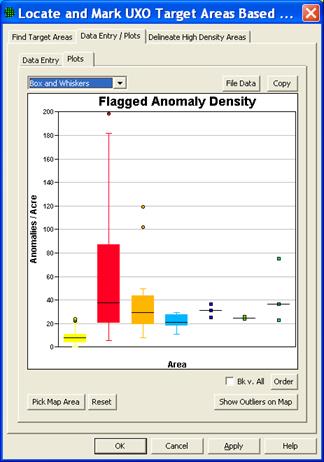
Figure 7.32.  Box and whisker plot showing result from target area delineation.

7.5 Assess Probability of Target Traversal Based on Actual Transect Pattern

By selecting Sampling Goals > Find Target Areas and Analyze Survey Results (UXO) > Assess probability of target area traversal based on actual transect pattern, the user can apply the actual transect pattern applied at a site and determine the probability that a target area of a specified size would be traversed by this pattern.  This transect pattern application is done by a Monte Carlo simulation in which each iteration randomly places the specified target area and determines if any transects traverse it. The "Post-Survey Probability of Traversal" dialog shown in Figure 7.33 uses the COG data to identify any locations on a site where a target area of the shape defined in the "Target Zone" tab could be located and not traversed. The number of iterations to run is set by the Number of Trials. The map in Figure 7.34 shows points (marked by small squares) where a target area of the size specified on the target zone tab could be located and not traversed. As the "Traversal Simulation" tab in Figure 7.33 shows, the transects within this area had an 82 percent probability of traversing all possible 500-ft-diameter target areas.

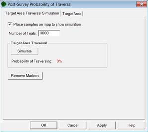
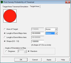
Figure 7.33. "Post-Survey Probability of Traversal" Dialog Used To Assess the Probability of Traversal Based on the Actual Transect Survey.  This dialog has the "Detection Simulation" tab (left) and the "Target Zone" tab (right).

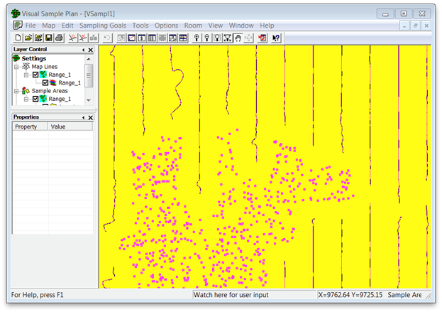
Figure 7.34. Example of the Map View After Clicking on the "Simulate" Button on the "Detection Simulation" Tab of the "Post-Survey Probability of Traversal" Dialog

7.6 Assess Degree of Confidence in UXO Presence

The UXO modules in VSP for Post Remediation Verification Sampling (UXO) assist in developing a sampling strategy to achieve high confidence that very few targets of interest (TOI) are present at a site or that very few detected anomalies at a site are TOI. The two modules can be used to determine the number of transects that should be surveyed to establish Y% confidence that at least X% of the transects at the site do not contain TOI, where Y, X, and the number of transects are entered by the user. The same method can be applied to detected anomalies to determine the number of detected anomalies to dig up to establish Y% confidence that at least X% of the detected anomaly locations do not contain TOI. 

In the Sampling Goal covered in this section, if there are TOI, they are limited and isolated objects not in any particular pattern. Two scenarios of interest are 1) a small UXO-remediated area where a survey is required to support a no-further-action (NFA) decision and 2) a very large unremediated area not expected to contain any TOI. In both scenarios, we assume the area of interest has a well-defined boundary. The area is divided into N non-overlapping, parallel transects with transect width equal to the width of the geophysical survey equipment. If N is large and only n of these transects can be surveyed, how should n be determined? This is similar to a compliance sampling problem in an industrial quality control setting where the goal is to determine if there are any defects before releasing a product. 

VSP addresses the variant of the problem where n must be of sufficient size to achieve a high confidence that few transects contain TOI. The method can also be applied to anomalies detected during a survey to achieve a high confidence that few detected anomalies are TOI.

7.6.1 Achieve High Confidence That Few Transects Contain UXO

Menu selection Sampling Goals > Post Remediation Verification Sampling (UXO) > Transect verification sampling brings up the dialog box in Figure 7.35 where the Transect Verification Sampling (left) and Transect Placement (right) tabs are shown. We enter a transect width of 2 m and a grid dimension (grid dimension and orientation is assumed to be aligned with the remediation grids) of 100 x 100 m. VSP informs us that there are N=62,050 total nonoverlapping transects within this Sample Area. The VSP user enters 99% as the minimum number of transects required to not contain one or more UXO (DQO input) and 95% as the confidence that this maximum percentage is not exceeded. VSP calculates that 298 of the 62,050 transects must be selected, using random sampling, and none of these transects can contain TOI in order to be "95% confident that at least 99% of the possible transects at the site do not contain TOI." The n=298 selected transects are randomly selected in length aggregated groups of 3 transects at 100 randomly selected locations. Attribute Compliance Sampling (ACS) (Schilling 1978; 1983, pages 475-482) is a statistical approach for establishing confidence in the cleanup effort. The sample size equation programmed into VSP for this problem is a method from Bowen and Bennett (1988). For extensive discussion of this problem and compliance sampling methods, consult VSP Help, Gilbert et al. (2003, Chapter 6) or Hathaway et al. (2008).  For Further help in this section refer to Presence/Absence Compliance Sampling.

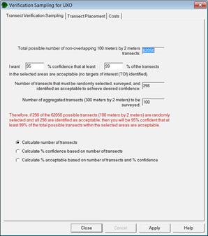
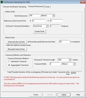
Figure 7.35. Dialog Input Box for Verification Sampling of TOI for the Transect Verification Sampling (left) and Transect Placement (right) tabs.

7.6.2 Achieve High Confidence That Few Anomalies are UXO

Menu selection Sampling Goals > Post Remediation Verification Sampling (UXO) > Anomaly verification sampling brings up the dialog box in Figure 7.36. Using the Millsite.dxf map and the large elliptical area selected as our Sample Area, we now include some data on anomaly locations. The 137 anomalies are shown either as small black "x" or small pink circles in Figure 7.36. The VSP user enters 90% as the minimum percent of anomalies required to not be TOI and 90% as the confidence that this maximum percentage is not exceeded.

VSP calculates that 39 of the 137 anomalies must be selected, using simple random sampling, and none of these anomalies can be UXO in order to be "90% confident that at least 90% of the possible anomalies at the site are not TOI. The n=39 randomly selected anomalies are shown on the map as small pink circles when the Apply button is pushed, as shown in Figure 7.35. The sample size equation programmed into VSP for this problem is a method from Bowen and Bennett (1988). 

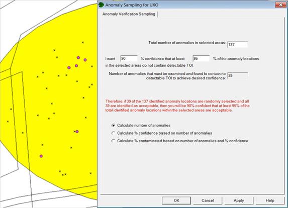
Figure 7.36. Dialog Input Box for Anomaly Sampling for UXO and Map of Sample Area with Anomalies Selected

Previous Next

References