Because the kriging algorithm requires a positive definite model of spatial variability, the experimental variogram cannot be used directly. Instead, a model must be fitted to the data to approximately describe the spatial continuity of the data. Certain models (i.e., mathematical functions) that are known to be positive definite are used in the modeling step.
The figure above shows an experimental variogram with a variogram model fitted to it. Each red square is a lag of the experimental variogram. The x-axis represents the distance between pairs of points, and the y-axis represents the calculated value of the variogram, where a greater value indicates less correlation between pairs of points. This particular variogram shows a spatial relationship well suited for geostatistical analysis since pairs of points are more correlated the closer they are together and become less correlated the greater the distance between points.
This graphic also illustrates three important parameters that control the fit of the variogram model. The nugget is the y-intercept of the variogram. In practical terms, the nugget represents the small-scale variability of the data. A portion of that short range variability can be the result of measurement error. The range is the distance after which the variogram levels off. The physical meaning of the range is that pairs of points that are this distance or greater apart are not spatially correlated. The sill is the total variance contribution, or the maximum variability between pairs of points.
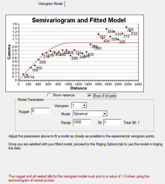
VSP can display the number of pairs that went into calculating each variogram lag. There should be at least 30 pairs for each variogram point, if there are fewer this could indicate that the distance between lags should be increased, so that more pairs are included in each lag.
The model type, nugget, sill and range can all be modified to fit the variogram model. Primary importance should be given to matching the slope for the first several reliable lags.
| Nugget: | Related to the amount of short range variability in the data. Choose a value for the best fit with the first few empirical variogram points. A nugget that's large relative to the sill is problematic and could indicate too much noise and not enough spatial correlation. |
| Model type: | See Deutsch & Journel for the details of these models. Spherical and exponential are most widely used. |
| Range: | The distance after which data are no longer correlated . About the distance where the variogram levels off to the sill. |
| Sill: | The sill is the total variance where the empirical variogram appears to level off, and is the sum of the nugget plus the sills of each nested structure. Variogram points above the sill indicate negative spatial correlation, while points below the sill indicate positive correlation . Can use the variance of data as a reasonable default. The variogram may not exhibit a sill if trends are present in the data. In that case, geostatistical analysis should proceed with caution, and at the least, ordinary kriging should be used for mapping. |
| Variogram number: | By default a single variogram model is used, but up to three can be nested to more accurately fit a model to the data. In cases where nested scales of spatial continuity appear to be present, it is best to attempt to determine the scientific reason for the multiple nested models (e.g., a short range might be related to the average dimensions of point bars, with a longer range related to the dimensions of a flood plain in which the point bars are distributed). |
Cameron, K, and P Hunter. 2002. Using Spatial Models and Kriging Techniques to Optimize Long-Term Ground-Water Monitoring Networks: A Case Study. Environmetrics 13:629-59.
Deutsch, C.V. and A.G. Journel. 1998. GSLIB Geostatistical Software Library and User's Guide, 2nd Edition, Applied Geostatistics Series, Oxford University Press, Inc. New York, NY.
Gilbert, RO. 1987. Statistical Methods for Environmental Pollution Monitoring. Van Nostrand Reinhold, New York.
Isaaks, EH, and RM Srivastava. 1989. An Introduction to Applied Geostatistics. Oxford University Press, New York.
Webster, R, and MA Oliver. 1993. How Large a Sample Is Needed to Estimate the Regional Variogram Adequately? . Geostatistics Troia '92 , ed. A Soares, Vol 1, pp. 155-66. Kluwer Academic Publishers, Dordrecht.