The temporal redundancy module in VSP provides methods for examination of the temporal spacing of observations. The object of the module is to identify a technically defensible temporal spacing. There are two different sampling goals that are addressed here. One of the main goals is determining if fewer observations could be used to characterize the contaminant concentrations at a well over time. A second objective that is sometimes needed is to identify the minimum temporal spacing between observations so that they are independent from one another. Methods are included in the module to address both objectives.
Before performing the analysis, the user may wish to clean the data. The Data Preparation tab in the Temporal Redundancy module includes tools to select wells for inclusion in the analysis, and to remove large temporal gaps and outliers that may be present in the data.
The iterative thinning approach is based on an algorithm published by Cameron (2004). The goal of the algorithm is simple, yet elegant: identify the frequency of sampling required to reproduce the temporal trend of the full data set. The trend may include simple upward or downward trends, but the algorithm also allows reproduction of more complex patterns, e.g., cyclical patterns related to seasonal variations in concentration.
The median temporal sample spacing between historical observations is first calculated and used as the baseline sample spacing. The iterative thinning algorithm uses the Lowess algorithm to fit a smooth trend and confidence bands (Cleveland 1979) around the full temporal data set. A default bandwidth of 0.5 is used. See LOWESS Plots for information on the equations used to fit the smooth trend and calculate the confidence bands around that trend. A percentage of the data points are removed from the data set and Lowess is used with the same bandwidth to fit a smooth trend to the reduced data set.
The ability of the reduced data set to reproduce the temporal trends in the full data set is evaluated by calculating the percentage of the data points on the trend for the reduced data set that fall within the 90% confidence interval established using the full data set. Increasing numbers of data points are removed from the data set and each of the reduced data sets is evaluated for their ability to reproduce the trend observed in the full data set. A default level of 75% of the points on the trend for the reduced data falling within the confidence limits around the original trend is deemed acceptable (Cameron 2004). In order to guard against artifacts that might arise from the selection of a single set of data points to remove, the iterative removal process is repeated a large number of times (default number of iterations is 500). The proportion of data that can be removed while still reproducing the temporal trend of the full data set is used to estimate an optimal sampling frequency.
The use of variogram analysis for analysis of temporal redundancy has been discussed by several authors, including Tuckfield (1994), Cameron and Hunter (2002), and Cameron (2004). The first step is to calculate a temporal variogram for well concentrations, and then fit a variogram model to the experimental variogram. Given the definition of the range of the variogram model as the lag distance beyond which data are no longer correlated, the variogram range was proposed by Tuckfield (1994) as an estimate of a technically defensible sampling frequency.
It should be noted that the goal of that approach was to provide sets of independent samples that could be used for credible comparisons (e.g., hypothesis testing) of up gradient and down gradient wells (Tuckfield 1994). This would require sampling that would be no more frequent than the temporal variogram range, so that independent samples would be obtained. This is a valid sampling design goal and for that reason, the use of variogram analysis is a valid approach for identifying a defensible temporal sampling frequency. However, it should be noted that the use of the temporal variogram approach would not define a sampling frequency that would be best for identifying any temporal trends in the data. If that is the goal of the analysis, then the iterative thinning approach described above would be more appropriate. Based on comparisons with data from a large number of wells from different contaminated locations, the optimal sampling frequency identified by the iterative thinning approach is usually much more frequent than that identified by the variogram range.
The temporal redundancy module includes several steps:
May remove outliers based on time gaps or extreme values
Iterative thinning
Variogram analysis
Before beginning, the data should be examined to ensure that the data are appropriate for temporal redundancy analysis. The Data Preparation tab will exclude all wells with less than 10 observations by default. Ten wells are usually sufficient for analysis by iterative thinning. However, more observations would be needed for variogram analysis, usually on the order of 20-30 observations, depending on the temporal spacing. If variogram analysis will be the primary tool, the user may want to exclude wells with short time series from the analysis.
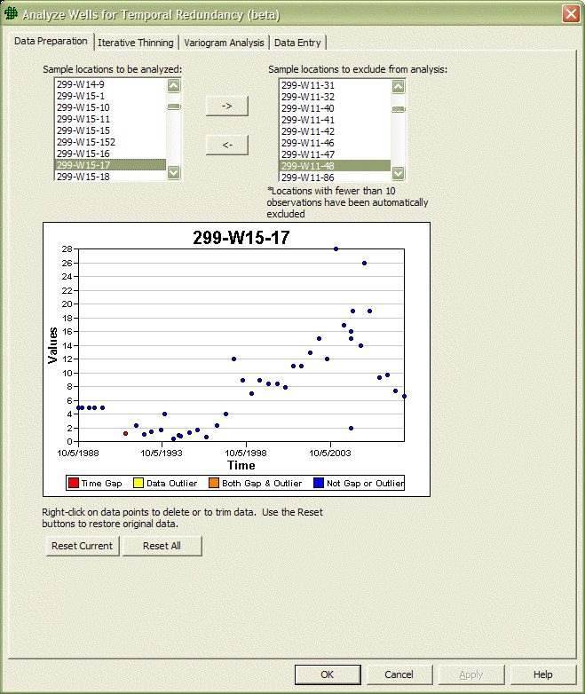
The Data Preparation tab allows the user to examine plots of the data to ensure that large time gaps, outliers, or other problem data are not present. For example, in the following figure, there is a gap in time between the fifth and sixth observations, identified by the program marking the sixth observation with a red circle. In addition, it appears that the first five observations were all at a detection limit. If the user right clicks on any data point, a menu is brought up that allows the user to eliminate a data point, all data before the data point, or all data after a data point. In this case, it might be appropriate to remove all data prior to the sixth observation.
As discussed above, the main choice to be made is whether to identify a temporal sampling plan that will allow reproduction of trends seen in the data, or to identify a temporal spacing that should be sufficient to ensure that samples are independent of one another. If the first goal is required, perform iterative thinning, otherwise perform a temporal variogram analysis.
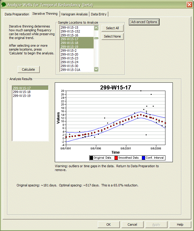
On the iterative thinning tab, the user first chooses which locations to analyze from the list of available wells. If the user then hits the Calculate button, the iterative thinning is performed for each of the selected wells. The results for each well can be viewed by selecting the well from the list in the Analysis Results.
The display of the results for each well shows the original data, the smoothed curve fit to the data, and a confidence interval around the smoothed curve. The default confidence interval is a 90% confidence interval.
Beneath the graph for each well will be a statement on the original spacing, the optimal spacing based on the parameters that were selected, and the reduction in the percentage of samples that would result at the optimal spacing.
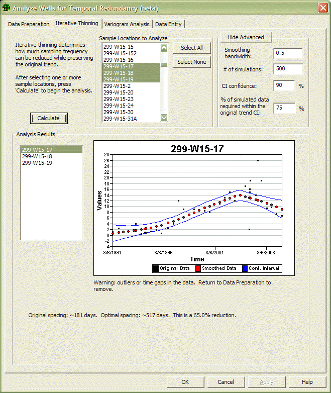
The user can also modify the default parameters used in performing the iterative thinning analysis. By clicking on the Advanced Options button, the user will be presented with the default settings, and can modify them, if desired.
Smoothing bandwidth
Related to the width of the smoothing window used in the Lowess smoother. Default is 0.5, as recommended by Cleveland (1979). Normally set between 0.2 and 0.8. Smaller bandwidths result in less smoothing of the trend, while wider bandwidths result in greater smoothing. The choice of bandwidth should also reflect the amount of data available. Small bandwidths should not be used with sparse time series.
# simulations
The number of Monte Carlo simulations to perform. In each Monte Carlo simulation a different set of randomly selected samples would be deleted from the base case. Default is 500 simulations, a smaller number would reduce the computational time.
CI confidence
The width of the confidence interval around the smooth trend. Default is set to a 90% confidence interval. The use of a wider confidence interval (e.g., a 95% CI) will make it more likely that the smooth trend fit to a reduced dataset will fall within the chosen CI around the base smooth trend, and thus result in a longer optimal spacing interval. The choice of CI will be documented in the report file.
% of simulated data required within the original trend CI
The default for the percentage of the simulated trend falling within the original trend CI is 75% (Cameron 2004). The choice of a smaller percentage will increase the optimal sample spacing. The percentage chosen will be documented in the report file.
The objective of the temporal variogram analysis is to identify the range of the variogram model that best fits the experimental variogram. The model type, nugget, sill and range can all be modified to fit the experimental variogram. If a nested model is required (i.e., one showing multiple structures), the range of interest will be the longest range identified. If an increasing or decreasing trend is present in the concentration data, then the variogram may increase without breaking over into a sill. In that case, the variance of the data can be used to identify the sill that must be reached by the model, so that a range can be identified. The range can then be used as a minimum estimate of the spacing between well samples that would ensure independence of the samples. A brief description of the parameters of the variogram model follow:
Related to the amount of short range variability in the data. Choose a value for the best fit with the first few empirical variogram points. A nugget that's large relative to the sill is problematic and could indicate too much noise and not enough temporal correlation.
See Deutsch & Journel or Isaaks and Srivastava for the details of these models. Spherical and exponential models are most widely used.
The time after which data are no longer correlated . Approximately the lag spacing where the variogram levels off to the sill.
The sill is the total variance where the empirical variogram appears to level off, and is the sum of the nugget plus the sills of each nested structure. Variogram points above the sill indicate negative temporal correlation, while points below the sill indicate positive correlation . The variogram may not exhibit a sill if trends are present in the data. In that case, one can use the variance of the data as a reasonable default for the sill.
By default a single variogram model is used, but up to three can be nested to more accurately fit a model to the data. In cases where nested scales of temporal continuity appear to be present, it is best to attempt to determine the scientific reason for the multiple nested models (e.g., a short range might be related to daily or other short term variations, with a longer range related to seasonal effects or changes in concentration due to migration of the plume).
Cameron, K. 2004. Better Optimization of Long-Term Monitoring Networks. Bioremediation Journal 8:89-107.
Cameron, K, and P Hunter. 2002. Using Spatial Models and Kriging Techniques to Optimize Long-Term Ground-Water Monitoring Networks: A Case Study. Environmetrics 13:629-59.
Cleveland W.S. 1979. Robust Locally Weighted Regression and Smoothing Scatterplots. Journal of the American Statistical Association, Vol. 74, No. 368. p. 829-836.
Deutsch, C.V. and A.G. Journel. 1998. GSLIB Geostatistical Software Library and User's Guide, 2nd Edition, Applied Geostatistics Series, Oxford University Press, Inc. New York, NY.
Isaaks, EH, and RM Srivastava. 1989. An Introduction to Applied Geostatistics. Oxford University Press, New York.
Tuckfield, RC. 1994. Estimating an Appropriate Sampling Frequency for Monitoring Ground Water Well Contamination. Presented at International Nuclear Materials Management (INMM) Annual Meeting: Naples. Available through DOE Office of Scientific and Technical Information, http://www.osti.gov/bridge//product.biblio.jsp?query_id=1&page=0&osti_id=10177871.