This tool provides several methods for creating simple interpolated maps of contaminant concentration across a site. These methods are similar to the geostatistical analysis tool in that they use previously sampled locations to estimate concentration values over a regular grid of locations in the sample area. However the methods used in this tool do not use a model of the underlying spatial correlation to improve the interpolation. This means that the resulting spatial maps may not be as accurate as a properly created geostatistical map, but it also means that the parameters and calculations necessary to create the interpolated maps are much simpler.
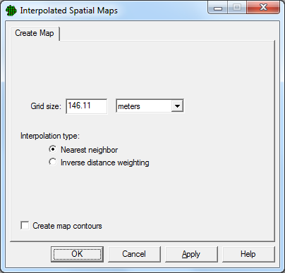
The first step in creating an interpolated map is to specify the size of the gridded estimates. A smaller grid size will result in a map with finer resolution but will take longer to calculate. The default grid size is1/30th of the site size, where the site size is the smallest of the length or the width of the site.
VSP then will fill in concentration values for those grid cells where there are no measurements present based on the existing measurement values using one of two interpolation methods.
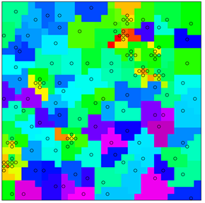
The simplest interpolation method is nearest neighbor interpolation. Each grid on the map is filled in with the value of the closest existing sample location. This isn’t truly “interpolating” but it provides an extremely quick way to visualize contaminant spread in a sample area even for very large areas or many existing sample values.
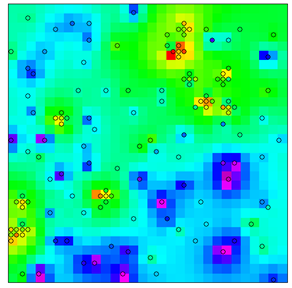
Inverse distance weighting estimates values for a particular grid location by calculating a weighted average using existing sample values located within a certain radius. The values are weighted according to the distance from the grid location to be estimated so that closer values are given more weight than values further away.
The weighting function used by VSP is \(w_x(g) = \frac{1}{d(g,x)^2} \) where \(d(g,x)\) is the Euclidian distance between points \(g\) and \(x\). The default search radius is 10 times the site size, where the site size is the smallest of the length or the width of the site, and any point \(x\) that is further than that distance from \(g\) will not be included in calculating the interpolated value for \(g\).
The interpolated value \(v\) at each grid cell location \(g\) is therefore calculated by the following function:
\begin{equation}v(g)=\sum_{i=0}^N\frac{\frac1{d(g,x_i)^2}x_i}{\sum_{j=0}^N\frac1{d(g,x_j)^2}}\end{equation}
where \(x_0,x_1,...x_N\) are the existing sample locations.
The resulting interpolated maps will be displayed on the map after pressing OK or Apply, and can be controlled in the Raster Data Layers section in the Layer Control Bar.
The color scale for the maps can be modified by right-clicking on the legend on the map. See Color Legends help for more details.