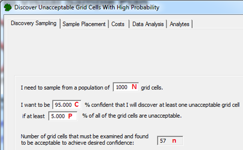
The objective of this design is to discover, with high probability, the presence of unacceptable grid cells if they exist. For example, if the purpose the sampling were to detect the presence of contamination - and assuming that, for each sample, the probability of a false negative is zero - this design could be used to answer the following question: If 1% of the decision area contained contamination, how many randomly located samples would I need to take to discover that contamination with 95% probability?
The following discussion is presented in terms of environmental sampling conducted within a decision area (such as room or collection of rooms within a building). However, this methodology is equally applicable to the sampling of any finite population of items, in which case the decision area is analogous to the population of items and the grid cell sampling locations are analogous to the individual items that will be sampled.
The hypergeometric model used in this design requires that each sample result be categorized as a binary outcome, such as 1) the presence or absence of a particular quality, 2) a sample result being acceptable or unacceptable as defined by an action level threshold, 3) contamination being detected or not detected, etc. This statistical model presented here is an alternative interpretation of the same hypergeometric model used in Compliance Sampling (Schilling and Neubauer 2009) and Accept on zero attribute compliance sampling (AOZ-ACS) (Squeglia, 1994; Bowen and Bennett, 1988). Instead of using a test of hypothesis as the basis for the sampling design, the discovery sampling model consists of calculating the probability that at least one of the grid cells in the random sample will be unacceptable, if the percentage of the population that is unacceptable is at least \(P\) x 100%.
Discovery sampling requires all surfaces in the decision area be divided into non-overlapping, equal-size grid cells of specified size that correspond to the sampling methodology, e.g., 10cm x 10 cm. The method may be used outdoors if the decision area can be divided into grid cells. The size of the grid cell should correspond to the footprint of the sampling methodology (i.e. the area sampled by the swab, wipe or vacuum). If more than one sampling methodology is to be employed in a decision area, the size of the grid cell should be chosen to match the sampling methodology with the smallest footprint. The location of samples that will be taken using methodologies with larger footprints should be assigned in a consistent fashion, e.g. the sample is centered on the smaller grid cell that was assigned by VSP, or the upper-left corner of the larger sample is aligned with the upper-left corner of the grid cell assigned by VSP, etc. While this approach to multiple sampling methodologies is conservative, it ensures that the desired confidence level is preserved.
Symbol |
Definition |
Range |
\(N\) |
The total number of grid cells in the decision area (i.e. target population) |
\(N\) \(\geq\) \(1\) |
\(n\) |
The number of grid cells that are selected using random sampling that will be measured or inspected. The number n is computed in VSP as described below. |
\(1 \leq n \leq N\) |
\(D\) |
The true number of unacceptable grids cells in the decision area |
\(1\) \(\leq\) \(D\) \(\leq\) \(N\) |
\(X\) |
The number of unacceptable grids cells observed in the sample results |
\(0\) \(\leq\) \(X\) \(\leq\) \(N\) |
\(C\) |
The desired confidence level, i.e., the probability of selecting at least one unacceptable grid cell, given that at least \(P\) x 100% of the grid cells in the population are unacceptable |
\(0\) \(\lt\) \(C\) \(\leq\) \(1\) |
\(P\) |
The smallest hypothetical fraction of unacceptable grid cells that we wish to discover |
\(\frac{1}{N}\) \(\leq\) \(P\) \(\leq\) \(1\) |
\(V\) |
The smallest hypothetical (and possibly fractional) number of unacceptable grid cells that we wish to discover, defined as \(V\) = \(P\)\(N\) |
\(1\) \(\leq\) \(V\) \(\leq\) \(N\) |
\(U\) |
The smallest whole number of hypothetical unacceptable grid cells. Specifically, \(U =\lceil V \rceil\), where \(\lceil V \rceil\) denotes the ceiling of \(V\), i.e., if \(V\) is not integer-valued, then round up to the nearest integer. |
\(1\) \(\leq\) \(U\) \(\leq\) \(N\) |
The discovery sampling design results in the following confidence statement:
If at least \(P\) x 100% of the population is unacceptable, the probability of discovering at least one unacceptable grid cell with a random sample of size n is at least \(C\) x 100%.
Because the hypergeometric model for discovery sampling is essentially the same as that used for compliance sampling, if, after sampling, none of the \(n\) grid units are unacceptable, then one may conclude with \(C\) x 100% confidence that at least \((1 - P)\) x 100% of the decision area is acceptable.
The required inputs for this design and their relationship to the preceding definitions are illustrated in Figure 1.
The size of the grid unit has been determined to be appropriate for the measurement (inspection) method to be performed. For example, an appropriate grid unit size might be a 10cm by 10cm surface area.
The total number of grid units in the decision area, \(N\), is known.
All \(N\) grid units are the same size.
\(n\) of the \(N\) grid units are selected using random sampling.
Each of the \(n\) grid units is measured or inspected using an approved method.
Each sample is correctly classified as being acceptable or unacceptable (no false positives or false negatives).
We want to identify the smallest value of \(n\) that satisfies the confidence function:
$$C \leq P(X \gt 0|D=U)$$
\begin{equation} = 1-P(X=0|D=U) \end{equation}
where \(X\) follows the hypergeometric distribution. Using the mass function of \(X\), we can express (1) as
\begin{equation} C \leq 1- \frac{\dbinom{U}{0}\dbinom{N-U}{n-0}}{\dbinom{N}{n}} =1-\frac{\Gamma (N-U+1) \Gamma (N-n+1)}{\Gamma (N-U-n+1) \Gamma (N+1)} \end{equation}
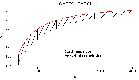
where \(\Gamma(x)=\int_{i=0}^\infty e^{-t}t^{x-1}dt\) is the gamma function. The sample size is the smallest integer-valued \(n\) which satisfies (2). While this sample size is an exact solution, it results in oscillating sample sizes as \(N\) increases, as illustrated in Figure 2 below. To avoid this phenomenon, VSP applies a continuous approximation to the sample size in (2) which ensures that as \(N\) increases, so does \(n\). This is accomplished by replacing \(U\) with \(V\) in equation (2). Specifically, define the approximate confidence function as
\begin{equation} f(n)= \begin{cases} 1-\frac{\Gamma(N-V+1)\Gamma(N-n+1)}{\Gamma(N-V-n+1)\Gamma(N+1)}, & \text{if \(n \lt N-U+1\)}\\ 1 & \text {otherwise}\\ \end{cases}\end{equation}
Note that unless \(V\) is integer valued, the definition of \(f\) is
slightly conservative, i.e. it results in a sample size with an achieved
confidence level slightly higher than the desired level, \(C\). Now define
\(f^{-1}(C)\) as the inverse of \(f(n)\) for \(1
\begin{equation} n= \begin{cases} 1, & \text{if \(f(1) \ge C\)}\\ N-U+1, & \text {if \(C = 1\)}\\ \lceil f^{-1}(C) \rceil & \text{otherwise}\\ \end{cases}\end{equation}
For a given \(n\), \(N\), and \(P\) (or \(U\)), the confidence is given by equation (3), except \(V\) is replaced with \(U=\lceil PN \rceil\), as follows:
\begin{equation} g(n,N,U) = \begin{cases} 1-\frac{\Gamma(N-U+1)\Gamma(N-n+1)}{\Gamma(N-U-n+1)\Gamma(N+1)}, & \text{if \(n \lt N-U+1\)}\\ 1 & \text {otherwise}\\ \end{cases}\end{equation}
When calculating the confidence, if the number of samples is large, i.e., \(n=N-U+1\), the achieved confidence is 100%. When this happens, it is possible that the hypothetical fraction of unacceptable grid cells that can be discovered with 100% confidence may actually be lower than the original desired value, \(P\). Because the smallest possible value of \(U\) that gives \(g(n,N,U)=1\) is \(N - n + 1\), the corresponding achieved value of \(P\) is \((N - n + 1) / N\).
The hypothetical fraction of unacceptable grid cells that may be discovered
in a population of size \(N\) with \(n\) samples and a desired confidence
level \(C\) can be obtained by numerically solving the right hand side
of (2) for \(P\). Let \(h(V)\) be equal to \(f(n)\) (equation (3)), except
now consider it a function of \(V\). Let \(h^{-1} (C)\) be the inverse
of \(h(V)\) for \(1
\begin{equation} U= \begin{cases} 1, & \text{if \(h(1) \ge C\)}\\ N-n+1, & \text {if \(C = 1\)}\\ \lceil h^{-1}(C) \rceil & \text{otherwise}\\ \end{cases}\end{equation}
and the achieved value of \(P\) is given by \(U/N\). When calculating \(P\), if the number of samples is large enough, i.e. \(n>CN\), the probability of discovering a single unacceptable grid cell will exceed the desired confidence level, \(C\). When this happens, the achieved confidence level for discovering a single unacceptable item can be calculated using equation (5): \(g(n,N,1)=1-\frac{(N-n)}{N}\).
When calculating the sample size, the confidence, or the fraction of unacceptable items that can be discovered, VSP will often return values of these parameters that are slightly different than the target values requested by the user. This occurs for a number of reasons. For example:
sample sizes are rounded up to the nearest integer, and this typically results in a slightly higher confidence than requested,
if the value of \(P\) results in a fractional value of \(V\), the achieved value of \(P\) (given by \(U/N)\), will be slightly higher than requested,
if a very large number of samples are taken, it is possible to achieve 100% confidence in discovering a smaller fraction of unacceptable items than originally requested, or
if a very large number of samples are taken, it is possible to discover a single unacceptable grid cell with a higher level of confidence than requested.
VSP reports the achieved values of all parameters in the red text that appears under the parameter inputs.
Bowen, M.W. and C.A. Bennett. 1988. Statistical Methods for Nuclear Material Management, NUREG/CR-4604, U.S. Nuclear Regulatory Commission, Washington, DC
Jaech, J.L. 1973. Statistical Methods in Nuclear Material Control, TID-26298, NTIS, Springfield, Virginia.
Schilling, E.G. and D.V. Neubauer. 2009. Acceptance Sampling in Quality Control, 2nd ed. CRC Press, Taylor & Francis Group, NY.
Squeglia, N.L. 1994. Zero Acceptance Number Sampling Plans. ASQ Quality Press, Milwaukee, WI.
Total Number of Grids Cells in Decision Area
Percentage of Decision Area that is Unacceptable
Data Analysis page