MARSSIM WRS Building Surfaces Gross Activity Design

The MARSSIM WRS (Wilcoxon Rank Sum) test is a two-sample test that compares the distribution of a set of measurements in a Survey Unit to that of a set of measurements in a Reference Area (i.e., background area). The MARSSIM WRS test is used to test whether the true median in a Survey Unit population is greater than the true median in a Reference Area population. The test compares medians of the two populations because the WRS is based on ranks rather than the measurements themselves. Note that if both the Survey Unit and Reference Area populations are symmetric, then the median and mean of each distribution are identical. In that special case the MARSSIM WRS test is comparing means. The assumption of symmetry and the appropriate use of the WRS test for final status surveys is discussed in Multi-Agency Radiation Survey and Site Investigation Manual (MARSSIM) (EPA 2000). This document is currently available at: https://www.epa.gov/radiation/multi-agency-radiation-survey-and-site-investigation-manual-marssim

Equations Used to Calculate Recommended Minimum Number of Samples

This design assume that you have more than one contaminant nuclide in the building surfaces study area and are interested in the gross activity of all radionuclides together. To enter the nuclides of concern, use the MARSSIM button on the Analyte page. The nuclides will have standard DCGLw values which may need to be modified for your particular application.

If you are an expert in MARSSIM designs, you can choose to enter all your own design parameters including:

Confidence%: Minimum desired probability of concluding the site is dirty if the true gross activity exceeds the DCGLw.

Beta%: Maximum desired probability of concluding the site is dirty if the true gross activity is less than the lower bound of the gray region.

Lower bound of the gray region (LBGR): A true gross activity value (below the DCGLw) above which you are willing to accept an increased risk of concluding the site is dirty.

Estimated standard deviation for the gross activity.

Estimated mean for the gross activity (in order to compute the power of the test).

As an alternative, you can have VSP assist you with the computation of the gross activity values. This approach will be emphasized here.

Activity Efficiency Calculations

Begin by entering the efficiency parameters for each of the nuclides along with the activity estimated mean and standard deviation for the total (gross) activity in the survey unit. The entry of values is illustrated below.

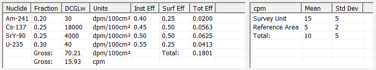
The left part of the entry area is dedicated to computing the detection efficiency. Efficiencies are necessary for converting between counts per minute (cpm) on the instrument and disintegration per minute over 100 square centimeters (dpm/100cm2), which is the common unit for a building surface DCGLw. First, the proportion of total Beta activity must be assigned to the nuclides and must sum to one. In this case, Am-241 accounts for 20% of the activity, Cs-137 accounts for 25%, SrY-90 for 25%, and U-235 accounts for 30% of total (gross) activity in the survey unit. Next, the instrument efficiency for each nuclide must be entered. This is the proportion of nuclide disintegrations (between 0.0 to 1.0) that is detected by the instrument. The surface efficiency must also be entered. This is the proportion of disintegrations that allow energy to escape the surface of the material to be detected by sensors. Surface efficiency is between 0.0 and 0.5. These efficiency values are obtained through calibration processes that are outside the scope of this document.

Total efficiency of each nuclide is computed as:

\(\text{Eff}_{\text{nuclide-total}} = \text{Fraction} \times \text{Eff}_{\text{instrument}} \times \text{Eff}_{\text{surface}}\)

All the total nuclide efficiencies are summed and reported as Total. In the example above, \(\text{Eff}_{\text{total}}\) is 0.1801.

Gross DCGLw in dpm/100cm2 units is computed as:

\begin{equation} DCGL_{Gross} = \frac{1}{\frac{f_1}{DCGL_1}+\frac{f_2}{DCGL_2}+..\frac{f_n}{DCGL_n}} \end{equation}

Gross DCGLw in dpm units can be computed as:

\begin{equation} DCGL_{dpm} = DCGL_{Gross} \times \frac{Area_{probe}}{100} \end{equation}

where \(Area_{probe}\) is the surface area of the instrument probe in square centimeters.

If all the efficiencies have been entered, Gross DCGLw in cpm units can be computed as:

\begin{equation} DCGL_{cpm} = DCGL_{Gross} \times Efficiency_{total} \times \frac{Area_{probe}}{100} \end{equation}

Activity Means and Standard Deviations

Now, the activity means and standard deviations for the emission group can be entered. If the probe area has been specified, you can enter the means and standard deviations in dpm. If all the efficiencies and the probe area have been specified, you can enter the mean and standard deviations in cpm. Otherwise, the mean and standard deviation must be entered in dpm/100cm2.

The expected mean and standard deviation (in the chosen units) for the survey unit must be entered.

The total mean is calculated as the Survey Unit Mean minus the Reference Area Mean. In this example, the total mean is: \(15 - 5 = 10 \text{cpm}\).

The total standard deviation is the largest of the Survey Unit Standard Deviation and the Reference Area Standard Deviation. In this example, it is 5 cpm.

Number of Samples

The standard deviation and mean values will be taken from the input table as described above. The gross activity DCGLw is taken from the efficiency calculates as detailed above. The units will match what you have chosen for entering the means and standard deviations above. This will normally be cpm.

You will need to enter the remaining design parameters:

Confidence%: Minimum desired probability of concluding the site is dirty if the true gross activity exceed the DCGLw.

Beta%: Maximum desired probability of concluding the site is dirty if the true gross activity is less than the lower bound of the gray region.

Lower bound of the gray region (LBGR): A true gross activity value (below the DCGLw) above which you are willing to accept an increased risk of concluding the site is dirty.

The number of samples is calculated using Equation (4) (EPA 2000, p. 5-28 and Gilbert et al. 2001, p. 3.12) and Equation (5) (Gilbert et al. 2001, p. 3.13).

\begin{equation} n+m = \dfrac{(z_{1-\alpha}+z_{1-\beta})^2}{3(P_{r}-0.5)^2} \end{equation}

\begin{equation} P_{r} = \Phi\Bigg(\dfrac{\Delta}{\sqrt{2}s_{\text{total}}}\Bigg) \end{equation}

where:

\(n+m\)	is the sum of the minimum number of study-site and reference-area samples, assuming n = m.
\(s_{\text{total}}\)	is the estimated standard deviation due to both sampling and measurement variability.
\(z_{1-\alpha}\)	is the value of the standard normal distribution for which the proportion of the distribution to the left of \(z_{1-\alpha}\) is \(1-\alpha\).
\(z_{1-\beta}\)	is the value of the standard normal distribution for which the proportion of the distribution to the left of \(z_{1-\beta}\) is \(1-\beta\).
\(\Delta\)	is the width of the gray region.
\(\alpha\)	is the probability of rejecting the null hypothesis when the null hypothesis is true.
\(\beta\)	is the probability of not rejecting the null hypothesis when the null hypothesis is false.
\({\Phi}_{\text{(x)}}\)	is the probability that a standard normal variate takes on a value \(\le\) x (CDF).

Statistical Assumptions

The assumptions associated with the formulas for computing the number of samples are:

1. although the population does not have to be normally distributed, the test statistic is approximately normally distributed,

2. the variances of the site and reference populations are equal,

3. the variance estimate, \(s^2\), is reasonable and representative of the populations being sampled,

4. the population values are not spatially or temporally correlated, and

5. the sampling locations will be selected randomly.

The first four assumptions will be assessed in a post data collection analysis. The last assumption is valid because the sample locations were selected using a random process.

References:

EPA. 2000. Multi-Agency Radiation Survey and Site Investigation Manual (MARSSIM). NUREG-1575, Rev. 1, EPA 402-R-97-016, Rev.1, DOE/EH-0624, Rev. 1. Environmental Protection Agency, Office of Research and Development, Quality Assurance Division, Washington DC.

Gilbert, RO, JR Davidson, JE Wilson, BA Pulsipher. 2001. Visual Sample Plan (VSP) models and code verification. PNNL-13450, Pacific Northwest National Laboratory, Richland, Washington.