The purpose of a one-sample t-test is to test a hypothesis involving the mean of a population against an Action Level. Please consult EPA's guidance document (Guidance for the Data Quality Objectives Process, 2006a) to put this test in the context of environmental decision making.
Before deciding to develop a sampling plan based on using the one-sample t-test, consider the assumptions and limitations involved. For example, this test assumes equality of variances (i.e. the standard deviations of the two populations are approximately equal). For a discussion of these assumptions, limitations, and the details of the test, please consult EPA's Data Quality Assessment: Statistical Methods for Practitioners (EPA 2006, pp. 66-71). This document, as well as the DQO guidance document, is currently available at: http://www.epa.gov/quality/qa_docs.html.
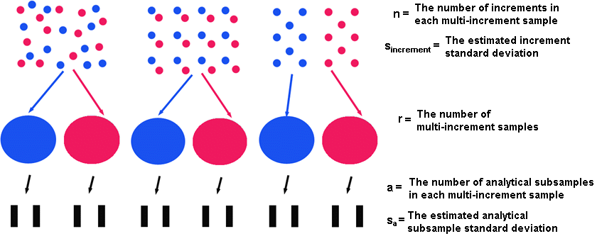
Multiple Increment (MI) sample designs (Composite sample designs) often arise because of the expense associated with analytical tests. A researcher would take \( n \) increments and combine them together in \( r \) groups (i.e. compositing or mixing soils together into one MI sample) and take measurements of each MI sample to get the average concentration for the combined increments. These measurements on each of the \( r \) MI samples are assumed to provide an accurate estimate of the mean concentration as if an average measurement was calculated from each of the individually measured increments.

The standard equation currently used in VSP to estimate the number of samples (\( n \)) which should be used to perform a one-sample t-test is shown first. This equation was obtained from (Gilbert, Wilson et al. 2005) and is also provided in the associated help files included with VSP. The equation is:
\begin{equation} n = \frac{(s_{total}^2)( Z_{1- \alpha } + Z_{1- \beta })^2}{\Delta^2} + 0.5Z_{1- \alpha}^2 \end{equation}
Where \( n \) = number of estimated samples in the survey unit, \( s_{total}^2 \) is the total variance between samples, \( Z \) represents a Normal(0,1) distribution, \( \Delta \) is the desired detectable difference, \( \beta \) is the probability of a Type II error, and \( \alpha \) is the probability of a Type I error.
The variance component in Equation 1 ( \( s_{total}^2 \) ) can be represented as
\begin{equation} s_{total}^2 = s_{sample}^2 + \frac{s_a^2}{a} \end{equation}
if there will be multiple analytical measurements (\( a \)) performed and there is an estimate for \( s_a^2 \). These equations are similar to the basic framework for the following equations that are used to calculate the total number of multiple increment samples to gather.
The general difference between Equation 1 and Equation 3 revolve around the fact that \( s_{total}^2 \) is a combination of three possible unknown sample elements. You may know the standard inputs for Equation 1, but you are left with how many replicate composite samples, increment samples, and repeated measurements to select (\( r,n,a \)) when you know all the other necessary inputs. Also, the \( n \) increments included in the multiple increment sample are not measured individually but are combined (through physical mixing) and measurements of the mixture are taken. Some different variance components that could be included in the total variation between composites include:
between increment variation
within increment variation
blending variation as the increments are mixed in the composite
measurement variation
as described in (Brown and Fisher 1972; Elder, Thompson et al. 1980; Rohlf, Akcakaya et al. 1996). The methods described below will account for between increment variation and subsample measurement variation. It should be explicitly noted that the blending variation is assumed to be very small. If the blending variation is too large the cost advantages of MI sampling will be lost (Hathaway et al. 2008). Thus, the overall variance between composites will be measured as
\begin{equation} s_{total}^2 = \frac{s_{analytical}^2}{a} + \frac{s_{increment}^2}{n} \end{equation}
Where \( s_{increment}^2 \) would be the same as \( s_{sample}^2 \) if each multiple increment sample were formed of \( n \) randomly selected increments of the total number of \( rn \) increments on the site of interest (See Figure above). If the \( n \) increments included in a specific multiple increment sample were not randomly selected from the entire site but selected from a smaller portion of the site (See Figure above) then \( s_{increment}^2 \leq s_{sample}^2 \) and \( s_{sample}^2 \) could be used as a conservative estimate, if no other estimate of \( s_{increment}^2 \) could be obtained.
\begin{equation} r = \frac{1}{\Delta^2} \left( \frac{s_{analytical}^2}{a} + \frac{s_{increment}^2}{n} \right) (t_{1- \alpha ,df} + t_{1- \beta ,df})^2 \end{equation}
where
\( r \) |
is the number of multiple increment (MI) samples, |
\( n \) |
is the number of increments per MI sample, |
\( s_{increment} \) |
is the estimated standard deviation of the between increment error, |
\( a \) |
is the number of analytical subsamples per MI sample, |
\( s_{analytical} \) |
is the estimated analytical subsample standard deviation, |
\( \Delta \) |
is the width of the gray region (delta), |
\( \alpha \) |
is the probability of rejecting the null hypothesis when the null hypothesis is true, |
\( \beta \) |
is the probability of accepting the null hypothesis when the null hypothesis is false, |
\( df \) |
is the degrees of freedom for the t-distribution which is \( r-1 \), |
\( t_{1- \alpha ,df} \) |
is the value of the t-distribution such that the proportion of the distribution less than \( t_{1- \alpha ,df} \) is \( 1- \alpha \), |
\( t_{1- \beta ,df} \) |
is the value of the standard normal distribution such that the proportion of the distribution less than \( Z_{1-\beta} \) is \( 1- \beta \). |
However Equation 4 attempts to estimate the number of MI samples (\(r\)) which depends on the number of increment samples (\(n\)) included in each composite sample and the number of analytical tests (\(a\)). The degrees of freedom associated with the t-distribution is now a function of \( r(df = r-1) \). The iterative process of estimating \( r \) can be used as described in VSP for the confidence interval on a mean (Gilbert 1987).
When \( a \) and \( n \) are fixed in the design dialog, Equation 4 is used to identify the number of MI samples (\(r\)) to gather. If \( a \) and \( n \) are not fixed in the design dialog, then VSP uses one of the following two methods described by Rohlf, Akcakaya et al. (1996).
If the option to find the optimal sampling plan for a fixed cost is selected the following iteration is used where \( C \) represents the cost associated with its respective label.
Calculate the ratio
\begin{equation} \sqrt{ \frac{s_a^2 C_{sample \, collection \, and \, combination}}{s_{increment}^2 C_{Individual \, Measurement}}} \end{equation}
For integer values of \( a \) and \( n \) where \( n = a/ratio \) compute
\begin{equation} r = \frac{C_{total}}{(nC_{sample \, collection \, and \, combination} + aC_{Individual \, Measurement} )} \end{equation}
requiring that \( r \geq 2 \).
Now for all good combinations of \( r, a \), and \(n\), calculate the smallest detectable difference by solving for \( \delta \) from Equation 4
Finally compute that actual total cost using
\begin{equation} Total Cost ( C_{total}) = r(n C_{sample \, collection \, and \, combination} + a C_{Individual \, Measurement}) \end{equation}
and summarize the top five smallest detectable difference options with their associated \( r , n , a \), and total cost.
If the option to find the minimum cost for a desired width of gray region (delta) is selected the following iteration is used where \( C \) represents the cost associated with its respective label.
Calculate the ratio
\begin{equation} \sqrt{ \frac{s_a^2 C_{sample \, collection \, and \, combination}}{s_{increment} C_{Individual \, Measurement}}} \end{equation}
For integer values of \( a \) and \( n \) where \( n = a /ratio \), compute the desired \( r \) from Equation 4. This is done iteratively because \( df \) is dependant on \( r \). This approach is detailed in Gilbert, Wilson et al. (2005). VSP requires that \( r \geq 2 \) .
For each plausible combination of \( r , a , n \) , calculate \( C_{total} \) from Equation 7.
Finally compute the actual detectable difference that could be obtained and summarize the top five least expensive options with their associated \( r, n , a \) , and detectable differences (\( \Delta \)).
The MI sample mean is normally distributed (this happens if the data are roughly symmetric or the total number of increments is more than 30; for extremely skewed data sets, additional samples may be required for the sample mean to be normally distributed).
The standard deviation estimates,\( s_{increment} \) and \( s_{analytical} \) , are reasonable and representative of the population being sampled.
The population values are not spatially or temporally correlated.
The sampling locations will be selected probabilistically.
The process of mixing increments in together in each MI sample is very good.
The number of MI samples must be two or greater.
The first three assumptions should be assessed in a post data collection analysis. The fourth assumption is valid because the gridded sample locations were selected based on a random start. It is recommended that the fifth assumption be examined during the study or in a previous study.
For more information concerning Multiple Increment Sampling, please refer to the VSP User's Guide.
Brown, G. H. and N. I. Fisher (1972). Subsampling a Mixture of Sampled Material. Technometrics 14(3): 663-&.
Elder, R. S., W. O. Thompson, et al. (1980). Properties of Composite Sampling Procedures. Technometrics 22(2): 179-186.
Gilbert, R., J. Wilson, et al. (2005). Technical Documentation and Verification for the Buildings Module in the Visual Sample Plan (VSP) Software. Richland, Pacific Northwest National Laboratory.
Gilbert, R. O. (1987). Statistical methods for environmental pollution monitoring. New York, Van Nostrand Reinhold Co.
Guenther, W. C. (1982). Normal Theory Sample-Size Formulas for Some Non-Normal Distributions. Communications in Statistics Part B-Simulation and Computation 11(6): 727-732.
Hathaway JE, G Schaalje, RO Gilbert, BA Pulsipher, and BD Matzke. 2008. Determining the Optimum Number of Increments in Composite Sampling. Environmental and Ecological Statistics. [Accepted]
Owen, D. B. (1962). Handbook of statistical tables. Reading, Mass., Addison-Wesley.
Rohlf, F. J., H. R. Akcakaya, et al. (1996). Optimizing composite sampling protocols. Environmental Science & Technology 30(10): 2899-2905.
Width of Gray Area (Delta) / LBGR / UBGR (when null hypothesis = "site is unacceptable")
Width of Gray Area (Delta) / LBGR / UBGR (when null hypothesis = "site is acceptable")
Type II Error Rate (Beta) (when null hypothesis = "site is unacceptable")
Type II Error Rate (Beta) (when null hypothesis = "site is acceptable")
Number of Analytical Subsamples Selector Estimated Increment Standard Deviation
Estimated Analytical Subsample Standard Deviation
Analytical Subsamples per Multiple Increment (MI) Sample