MARSSIM Building Surfaces Gross Activity Design

The MARSSIM Sign test is a one-sample, nonparametric statistical test used to determine compliance with a release criterion, i.e., the Weighted Derived Concentration Guidance Level (DCGLw) when the radionuclide of concern is not present in background. The purpose of a MARSSIM sign test is to test a hypothesis involving the true mean or median of a population against the DCGLw. Note that using this test for the mean assumes the distribution of the survey unit population is symmetrical. When the distribution of the population in the Survey Unit is symmetrical, the mean and the median are the same. When the distribution is not symmetrical, the Sign test is a true test for the median, and an approximate test for the mean. This assumption and the appropriate use of the sign test for final status surveys is discussed in Multi-Agency Radiation Survey and Site Investigation Manual (MARSSIM) (EPA 2000). This document is currently available at: https://www.epa.gov/radiation/multi-agency-radiation-survey-and-site-investigation-manual

This VSP module implements the functionality of the old COMPASS software from Oak Ridge Associated Universities (ORAU) / Oak Ridge Institute for Science and Education (ORISE).

Equations Used to Calculate Recommended Minimum Number of Samples

This design assume that you have more than one contaminant nuclide in the building surfaces study area and are interested in the gross activity of all radionuclides together. To enter the nuclides of concern, use the MARSSIM button on the Analyte page. The nuclides will have standard DCGLw values which may need to be modified for your particular application.

If you are an expert in MARSSIM designs, you can choose to enter all your own design parameters including:

Confidence%: Minimum desired probability of concluding the site is dirty if the true gross activity exceeds the DCGLw.

Beta%: Maximum desired probability of concluding the site is dirty if the true gross activity is less than the lower bound of the gray region.

Lower bound of the gray region (LBGR): A true gross activity value (below the DCGLw) above which you are willing to accept an increased risk of concluding the site is dirty.

Estimated standard deviation for the gross activity.

Estimated mean for the gross activity (in order to compute the power of the test).

As an alternative, you can have VSP assist you with the computation of the gross activity values. This approach will be emphasized here.

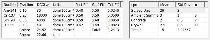
Activity Efficiency Calculations

Begin by entering the efficiency parameters for each of the nuclides along with the activity estimated mean and standard deviation for the total (gross) activity in the survey unit. The entry of values is illustrated below.

The left part of the entry area is dedicated to computing the detection efficiency. Efficiencies are necessary for converting between counts per minute (cpm) on the instrument and disintegration per minute over 100 square centimeters (dpm/100cm2), which is the common unit for a building surface DCGLw. First, the proportion of total Beta activity must be assigned to the nuclides and must sum to one. In this case, Am-241 accounts for 10% of the activity, Cs-137 accounts for 20%, SrY-90 for 30%, and U-235 accounts for 40% of total (gross) activity in the survey unit. Next, the instrument efficiency for each nuclide must be entered. This is the proportion of nuclide disintegrations (between 0.0 to 1.0) that is detected by the instrument. The surface efficiency must also be entered. This is the proportion of disintegrations that allow energy to escape the surface of the material to be detected by sensors. Surface efficiency is between 0.0 and 0.5. These efficiency values are obtained through calibration processes that are outside the scope of this document.

Total efficiency of each nuclide is computed as:

\(\text{Eff}_{\text{nuclide-total}} = \text{Fraction} \times \text{Eff}_{\text{instrument}} \times \text{Eff}_{\text{surface}}\)

All the total nuclide efficiencies are summed and reported as Total. In the example above, \(\text{Eff}_{\text{total}}\) is 0.2413.

Gross DCGLw in dpm/100cm2 units is computed as:

\begin{equation} DCGL_{Gross} = \frac{1}{\frac{f_1}{DCGL_1}+\frac{f_2}{DCGL_2}+..\frac{f_n}{DCGL_n}} \end{equation}

Gross DCGLw in dpm units can be computed as:

\begin{equation} DCGL_{dpm} = DCGL_{Gross} \times \frac{Area_{probe}}{100} \end{equation}

where \(Area_{probe}\) is the surface area of the instrument probe in square centimeters.

If all the efficiencies have been entered, Gross DCGLw in cpm units can be computed as:

\begin{equation} DCGL_{cpm} = DCGL_{Gross} \times Efficiency_{total} \times \frac{Area_{probe}}{100} \end{equation}

Activity Means and Standard Deviations (without background corrections)

Now, the activity mean and standard deviation can be entered. If the probe area has been specified, you can enter the mean and standard deviation in dpm. If the probe area and all of the efficiencies have been specified, you can enter the mean and standard deviation in cpm. Otherwise, the mean and standard deviation must be entered in dpm/100cm².

Activity Means and Standard Deviations (with background corrections)

The typical approach for analyzing survey units when background radiation is a concern involves comparing the survey unit measurement distribution to an appropriate background distribution using the WRS test. When the background radiation is coming from multiple distinct surface materials this approach can be problematic and dramatically increase the required number of samples. NUREG 1505 Chapter 12 provides and example highlighting these challenges and offers an alternative approach using paired measurements and conducting a sign test. The main idea in this approach is to appropriately adjust the survey unit measurements to account for background and then analyze the resulting values instead of comparing two distributions (survey unit and background). When using the sign test approach described in NUREG 1505 Chapter 12, some care needs to be taken as to how the background adjustment is computed and how this affects the underlying variance of the values used in the sign test. Though NUREG 1505 describes this as a paired observation approach, section 12.3 describes both a paired approach and an approach using average values from each material type. Using average values from each material type can often provide better precision than a paired approach, and thus VSP implements an approach using average values from each material type.

If you choose to use background corrections, you must enter estimated means, standard deviations and the sample size for each of the background factors (VSP uses a default sample size of 2). In this example, Ambient Gamma and two material specific backgrounds (Concrete and Drywall) have been specified. Background correction factors can be specified by clicking on the button labeled Bkg Corrections.

If background factors are used, the total mean is calculated as the Survey Unit Mean minus the Ambient Gamma Mean and the smallest Material Specific Background Mean. In this example, the total mean is: \(20 - 3 - 2 = 15 \text{ cpm}\).

The total standard deviation for each activity is calculated using propagation of errors formula combining the contributed variance from the Survey Unit, the Ambient Gamma, and the distinct materials present in the survey unit. This formula is a conservative version of the formula described in NUREG 1505 Ch.12. The adjusted standard deviations are computed by dividing the standard deviation by the square root of the number of samples (n) that were used to establish the standard deviation.

\begin{equation} S_{tot} = \sqrt{(S_{su})^2+\Big(\frac{S_{ag}}{\sqrt{n}}\Big)^2 +\Big(\frac{S_{mm}}{\sqrt{n}}\Big)^2} \end{equation}

Where \(S_{su}\) is the Survey Unit Standard Deviation, \(S_{ag}\) is the Ambient Gamma Standard Deviation and \(S_{mm}\) is the maximum (after adjustment) Material Specific Standard Deviation. In this example the adjusted standard deviation for concrete is \(\Big(\frac{0.5}{\sqrt{7}}\Big)=0.189\) and the adjusted standard deviation for drywall is \(\Big(\frac{0.6}{\sqrt{11}}\Big)=0.181\), so concrete will be used. The total standard deviation is \(\sqrt{3^2 + \Big(\frac{1}{\sqrt{8}}\Big)^2 + \Big(\frac{0.5}{\sqrt{7}}\Big)^2 }\) = \(\sqrt{9.1607} = 3.03 \text{cpm}\).

Number of Samples

The standard deviation and mean values will be taken from the input table as described above. The gross activity DCGLw is taken from the efficiency calculates as detailed above. The units will match what you have chosen for entering the means and standard deviations above. This will normally be cpm.

You will need to enter the remaining design parameters:

Confidence%: Minimum desired probability of concluding the site is dirty if the true gross activity exceed the DCGLw.

Beta%: Maximum desired probability of concluding the site is dirty if the true gross activity is less than the lower bound of the gray region.

Lower bound of the gray region (LBGR): A true gross activity value (below the DCGLw) above which you are willing to accept an increased risk of concluding the site is dirty.

The number of samples is calculated using Eq. (1) (EPA 2000, p. 5-33).

\begin{equation} n = \frac{(z_{1-\alpha}+z_{1-\beta})^2}{4(\text{Sign} P-0.5)^2} \quad \mbox{where} \quad \text{Sign} P = \Phi\Big(\frac{\Delta}{S_{\text{tot}}}\Big) \end{equation}

where:

\(n\)	is the recommended minimum sample size.
\(S_{\text{tot}}\)	is the estimated standard deviation for the total gross activity defined in equation (4) above.
\(z_{1-\alpha}\)	is the value of the standard normal distribution for which the proportion of the distribution to the left of \(z_{1-\alpha}\) is \(1-\alpha\).
\(z_{1-\beta}\)	is the value of the standard normal distribution for which the proportion of the distribution to the left of \(z_{1-\beta}\) is \(1-\beta\).
\(\Delta\)	is the width of the gray region.
\(\alpha\)	is the probability of rejecting the null hypothesis when the null hypothesis is true.
\(\beta\)	is the probability of not rejecting the null hypothesis when the null hypothesis is false.
\({\Phi}_{\text{(x)}}\)	is the probability that a standard normal variate takes on a value \(\le\) x (CDF).

Statistical Assumptions

The assumptions associated with the formulas for computing the number of samples are:

1. The computed sign test statistic is normally distributed.

2. The mean and standard deviation (\(S\)) estimates are reasonable and representative of the population being sampled.

3. The population values are not spatially or temporally correlated.

4. The sampling locations will be selected randomly.

The first three assumptions will be assessed in a post data collection analysis. The last assumptions is valid because the sample locations were selected using a random process.

References:

EPA. 2000. Multi-Agency Radiation Survey and Site Investigation Manual (MARSSIM). NUREG-1575, Rev. 1, EPA 402-R-97-016, Rev.1, DOE/EH-0624, Rev. 1. Environmental Protection Agency, Office of Research and Development, Quality Assurance Division, Washington DC.